Quantitative Methods
Serena DeStefani – Lecture 2 – 7/7/2020
Announcements
First HW due tomorrow morning before class:
- Upload answers on Sakai
- Email me a screenshot of your work
Please join Datacamp
Tutor available
Review
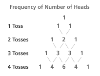
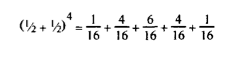
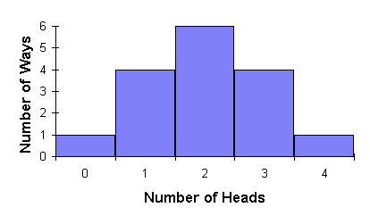
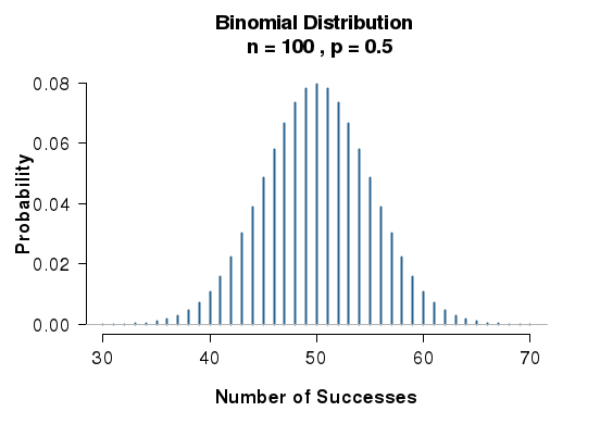
From the binomial expansion to the normal distribution
We can plot the frequency of getting heads on a histogram
Review
How to display and describe categorical data:
- Frequency tables
- Bar Charts
- Pie Charts
Review
How to compare categorical data:
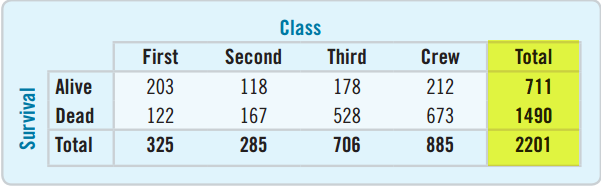
- Contingency tables
- Marginal distribution
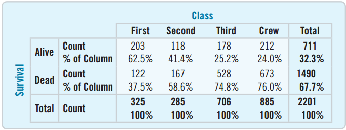
- Conditional distribution:
- percent of one variable satisfying the conditions of another
- can be organized by column or by row
Review
Independence: The distribution of one variable is the same for all categories of another.
There is no association between the two.
An association that holds for all of several groups can reverse direction when the data are combined to form a single group. This reversal is called Simpson’s paradox.
Chapter 3
Displaying and Summarizing Quantitative Data
- HISTOGRAMS -
Histogram: A chart that displays quantitative data
Great for seeing the distribution of the data
![]()
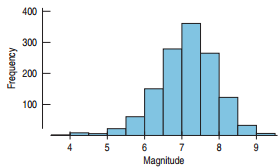
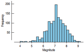
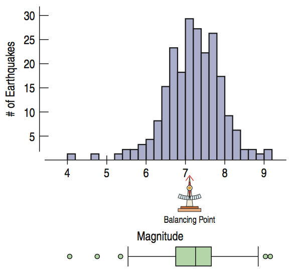
A histogram of tsunami generating earthquakes
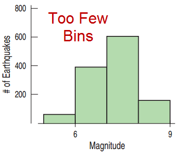
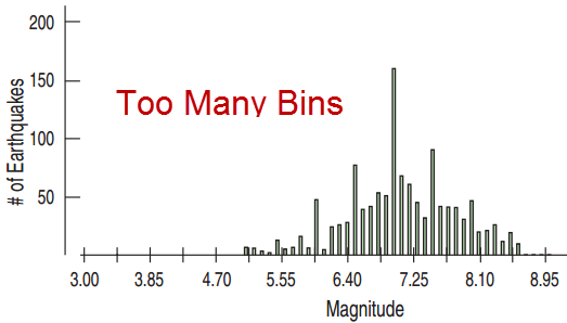
Choosing the Bin Width
Different bin widths tell different stories.
Relative Frequency Histograms
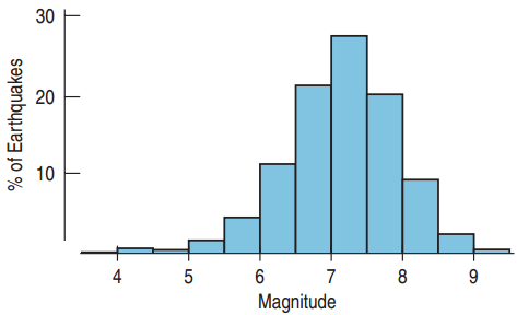
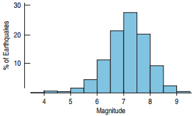
Relative Frequency Histogram
- The vertical axis represents the relative frequency, the frequency divided by the total.
Think Before you Draw
Is the variable quantitative? Is the answer to the survey question or result of the experiment a number whose units are known?
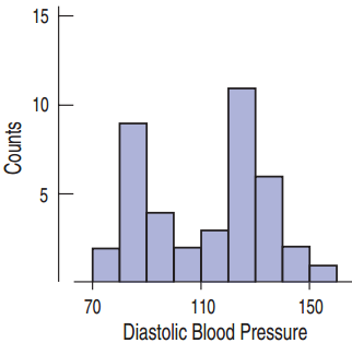
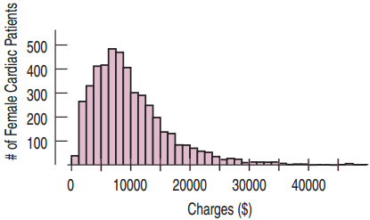
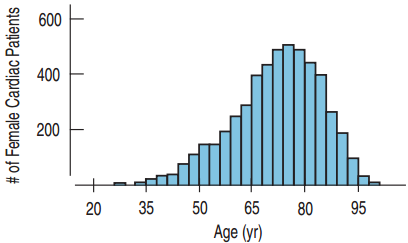
Shape: Modes
A Mode of a histogram is a hump or high-frequency bin.
Outliers
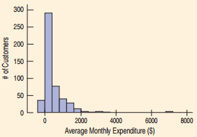
An Outlier is a data value that is far above or far below the rest of the data values.
![]()
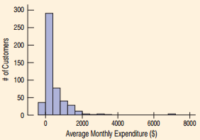
Example
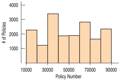
The histogram shows the amount of money spent by a credit card company’s customers. Describe and interpret the distribution.
- CENTER -
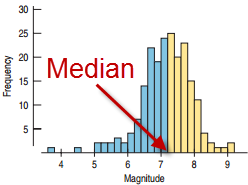
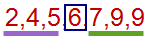
Median: The center of the data values
![]()
- SPREAD -
Locating the center is only part of the story
Range
The range is the difference between the maximum and minimum values.
\[\text{Range} = \text{Maximum} - \text{Minimum}\]
Percentiles and Quartiles
Percentiles divide the data into one hundred groups.
The \(n\)th percentile is the data value such that \(n\) percent of the data lies below that value.
- Median?
- first quartile (Q1).
- third quartile (Q3).
The Interquartile Range
The Interquartile Range (IQR) is the difference between the upper quartile and the lower quartile
\[\text{IQR} = Q3 - Q1\]
The Interquartile Range
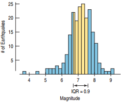
The Interquartile Range for earthquake causing tsunamis is 0.9.
The picture below shows the meaning of the IQR.
![]()
Benefits and Drawbacks of the IQR
- Outliers?
- Summary?
- What does it show?
- General audience?
5-Number Summary
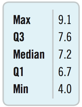
The 5-Number Summary provides a numerical description of the data. It consists of
- Minimum
- First Quartile (Q1)
- Median
- Third Quartile (Q3)
- Maximum
The list to the right shows the 5-Number Summary for the tsunami data.
Boxplots
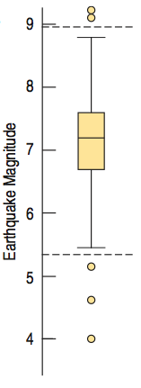
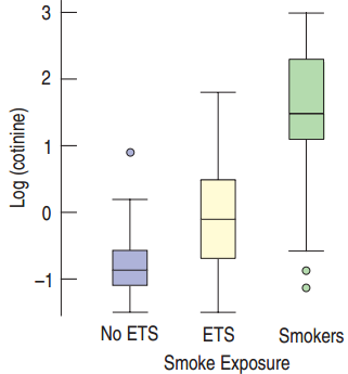
A Boxplot is a chart that displays the 5-Point Summary and the outliers.
- Box
- Fences
- Whiskers
- Median.
Finding the Fences
The lower fence is defined by: Lower Fence = Q1 – (1.5 × IQR)
The upper fence is defined by: Upper Fence = Q3 + (1.5 × IQR)
Tsunami Example: Q1 = 6.7, Q3 = 7.6
- IQR = 7.6 – 6.7 = 0.9
- Lower Fence = 6.7 – 1.5 × 0.9 = 5.35
- Upper Fence = 7.6 + 1.5 × 0.9 = 8.95
Step-by-Step Example of Shape, Center, Spread: Flight Cancellations
Question: How often are US flights cancelled?
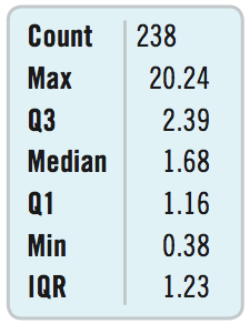
We have a dataset with flight cancellations by month
- Who? Months
- What? Percentage of Flights Cancelled at U.S. Airports
- When? 1994 – 2013
- Where? United States
- How? Bureau of Transportation Statistics Data
Flight Cancellations
Identify the Variable
- Percent of flight cancellations at U.S. airports
- Quantitative: Units are percentages.
How will the data be summarized?
- Histogram
- Numerical Summary
- Boxplot
Flight Cancellations
How is the data skewed?
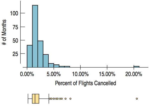
- Skewed to the Right: Can’t be a negative percent. Bad weather and other airport troubles can cause extreme cancellations.
What can we say about the IQR?
- IQR is small: 1.23%. Consistency among cancellation percents
Do we have an outlier?
- Extraordinary outlier at 20.2%: September 2001
Symmetric Distributions
A symmetric distribution is easier to describe
The Center of Symmetric Distributions: the Mean
The Mean is what most people think of as the average.
Add up all the numbers and divide by the number of numbers.
\[\bar{y} = \frac{\sum y}{n}\]
Recall that \(\sum\) means “Add them all.”
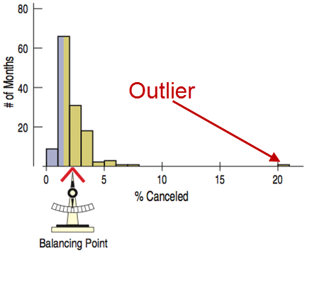
The Mean is the “Balancing Point”
If you put your finger on the mean, the histogram will balance perfectly.
The Mean Is Attracted to the Outlier
![]()
Why Use the Mean?
- Which one is easier to work with?
- Which one weights the data better?
- Symmetric data?
- Report both?
The Variance
\[s^2 = \frac{\sum \left(y - \bar{y}\right)^2}{n-1}\]
The variance is a measure of how far the data is spread out from the mean.
The difference from the mean is: \(y - \bar{y}\).
To make it positive, square it.
Then find the average of all of these distances, except instead of dividing by \(n\), divide by \(n - 1\).
Use \(s^2\) to represent the variance.
The variance will mostly be used to find the standard deviation \(s\) which is the square root of the variance.
Standard Deviation
The variance’s units are the square of the original units.
Taking the square root of the variance gives the standard deviation, which will have the same units as \(y\).
The standard deviation is a number that is close to the average distances that the \(y\) values are from the mean.
If data values are close to the mean (less spread out), then the standard deviation will be small.
If data values are far from the mean (more spread out), then the standard deviation will be large.
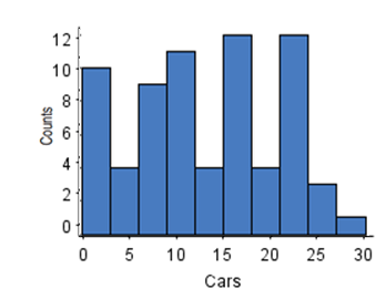
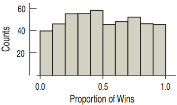
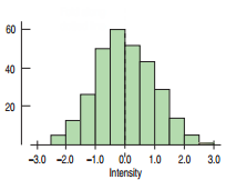
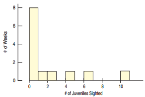
The Standard Deviation and Histograms
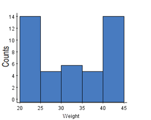
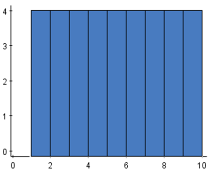
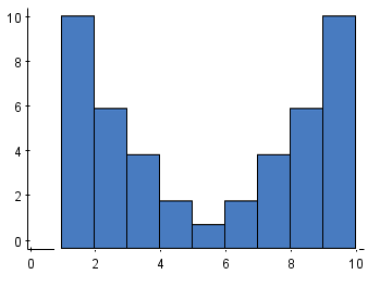
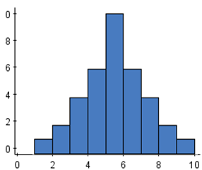
Order the histograms below from smallest standard deviation to largest standard deviation.
Summary
Histogram, Boxplot
Center and Spread
- if not symmetric?
- if symmetric?
- Unimodal symmetric data?
Unusual Features
- For multiple modes?
- Outliers?
Example: Fuel Efficiency
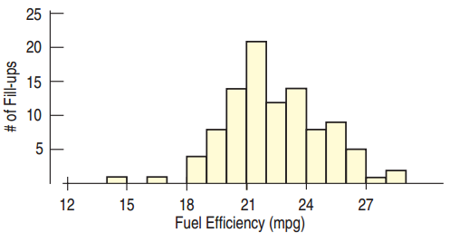
The car owner has checked the fuel efficiency each time he filled the tank of his new car. How would you describe the fuel efficiency?
Plan: Summarize the distribution of the car’s fuel efficiency.
Variable: mpg for the first 100 fill ups, Quantitative
Mechanics: show a histogram
- Fairly symmetric
- Low outlier
Fuel Efficiency Continued
Which to report?
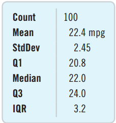
- The mean and median are close.
- Report the mean and standard deviation.
Conclusion
- Distribution is unimodal and symmetric.
- Mean is 22.4 mpg.
- Low outlier may be investigated, but limited effect on the mean
- \(s\) = 2.45; from one filling to the next, fuel efficiency differs from the mean by an average of about 2.45 mpg.
What Can Go Wrong?
Don’t make a histogram for categorical data.
Don’t look for shape, center, and spread for a bar chart.
Choose a bin width appropriate for the data.
What Can Go Wrong? Continued
Do a reality check
- Don’t blindly trust your calculator. For example, a mean student age of 193 years old is nonsense.
Sort before finding the median and percentiles.
- 315, 8, 2, 49, 97 does not have median of 2.
Don’t compute numerical summaries for a categorical variable.
- The mean Social Security number is meaningless.
What Can Go Wrong? Continued
Don’t report too many decimal places.
- Citing the mean fuel efficiency as 22.417822453 is going overboard.
Don’t round in the middle of a calculation.
For multiple modes, think about separating groups.
- Heights of people → Separate men and women
Beware of outliers, the mean and standard deviation are sensitive to outliers.
- Use a histogram or dotplot to ensure that the mean and standard deviation really do describe the data.
Chapter 4
Understanding and Comparing Distributions
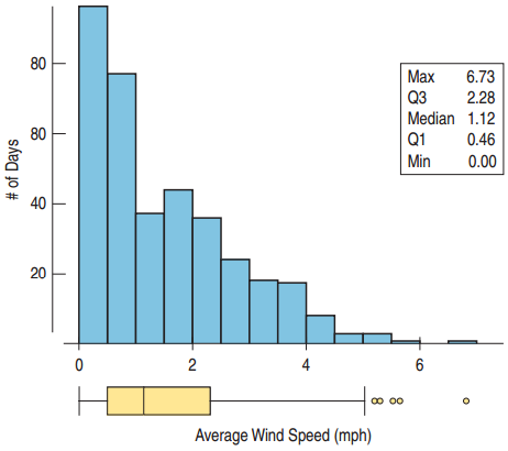
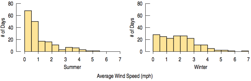
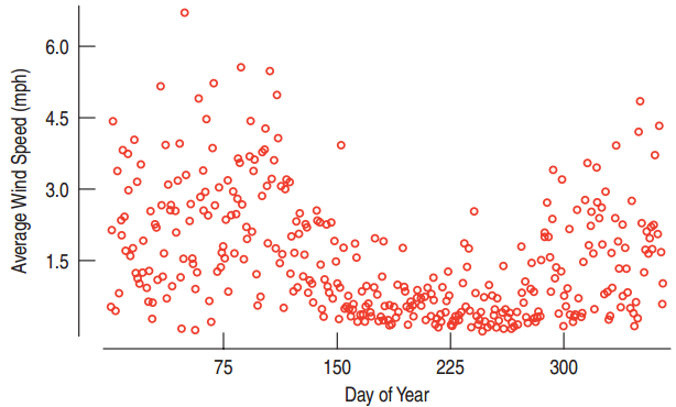
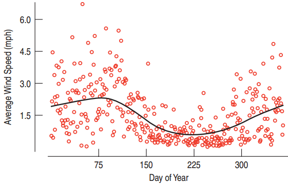
Wind Speeds in the Hopkins Memorial Forest
![]()
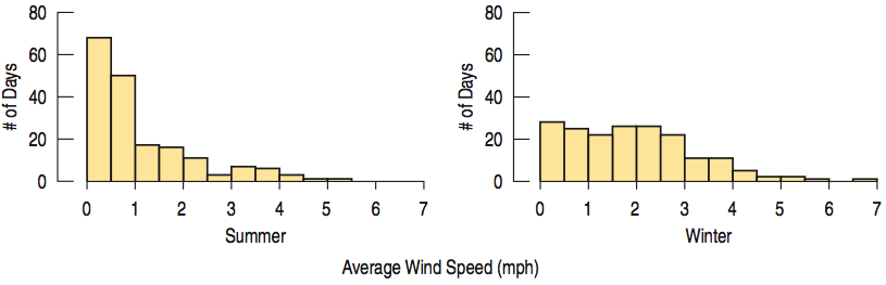
Comparing Seasons
![]()
Comparing Seasons (Continued)
![]()
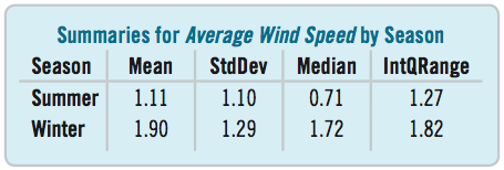
Comparing Seasons (Continued)
![]()
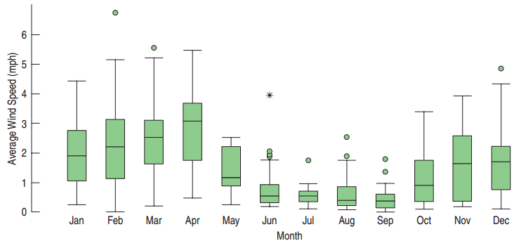
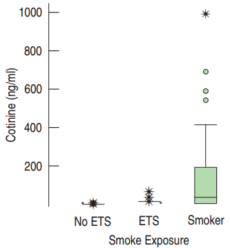
Using Boxplots for Comparisons
Are some months windier than others?
![]()
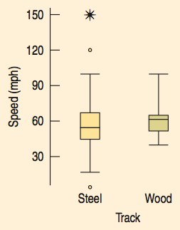
Wooden Vs. Steel
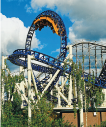
Which type of roller coaster is faster: steel or wooden?
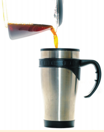
Please, No Cold Coffee!
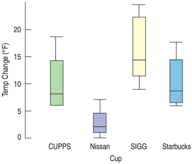
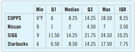
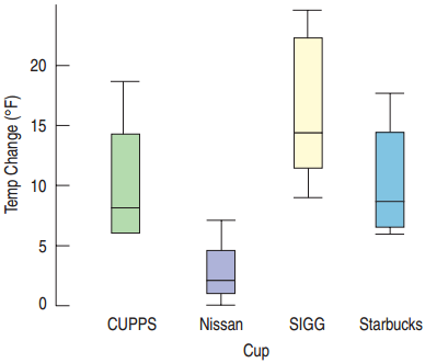
We want to compare which of 4 different coffee cups keeps the coffee hot.
Measure the temperature 30 minutes after being poured for each of the four types. Repeat the experiment 8 times.
- Plan: Compare the data sets for the four types.
- Variables: Quantitative – Temperature change of coffee
Conclusion
![]()
How to Approach Outliers
Check to see if there may have been an error in the data collection or data input.
- If the reported heights of students include a student that is 170 inches tall (14 feet), maybe that student was measured in centimeters.
Check to see if there was an extraordinary outcome.
- The median number of daily customers at the Punxsutawney, PA, gift store may be 42 with an IQR of 12, but on December 23rd, there were 831 customers.
Common Errors Causing an Outlier
- Transposing the digits
- A respondent not understanding the survey question
- Misreading results
- Confusion about units
- Cheating
The Outliers Can be the Most Interesting Data Values
Income Data:
Student Height:
- The basketball team’s center
Snowfall:
- The great blizzard of ’98
Exam Score:
Always comment on the outliers.
Timeplots
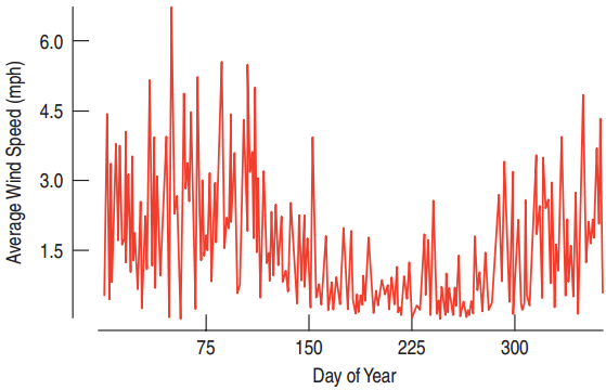
Timeplots display every data value on a timeline.
Connecting the Dots
![]()
Smoothing the Data
![]()
Lowess curve
Looking into the Future
Time plots can sometimes be used to predict future trends.
- Knowing that last summer was calmer than last winter can be used to make predictions about next summer and next winter.
Predicting the future with a time plot does not always work.
- Last year’s hurricane outlier will not tell you about a hurricane for this year.
- Stock prices cannot be predicted with a time plot.
- Roller coaster speeds will not increase forever.
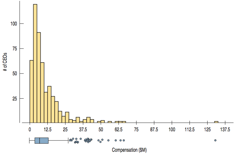
Trouble with Too Many Outliers
![]()
What Can Go Wrong?
Avoid inconsistent scales.
- Don’t try to compare one thing measured in feet to another measured in meters.
Label Clearly.
- Variables should be identified, and axes labeled.
Beware of Outliers!
- If the outliers are errors, remove them.
- Otherwise, consider presenting with and without the outliers.
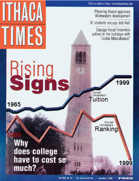
What’s Wrong With This?
![]()
Things to remember
Choose the right tool.
- Use histograms to compare two or three groups.
- Use boxplots to compare many groups.
Treat outliers with attention and care.
- Investigate if the outliers are errors or remarkable.
Use a timeplot to track trends over time.
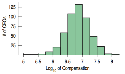
Re-express or transform data for better understanding.
- Can transform skewed distributions to symmetric ones
- Can help to compare spreads of different groups
Chapter 5
The Standard Deviation as a Ruler and the Normal Model
5.1
Standardizing with z-Scores
Comparing Athletes
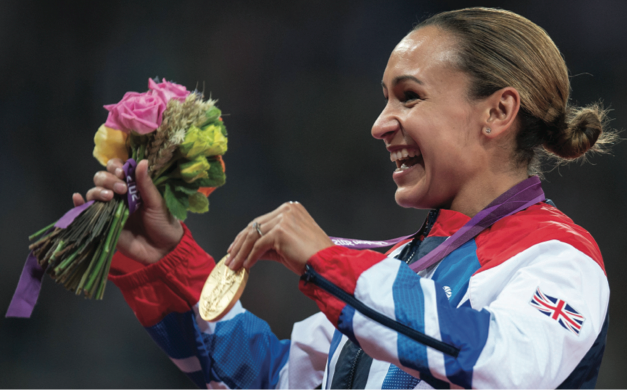
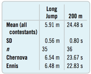
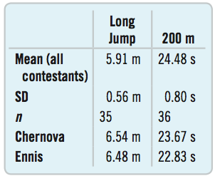
Chernova took the gold in the Olympics with a long jump of 6.545 m
- about 0.5 m farther than the mean distance.
Jessica Ennis won the 200 m run with a time of 22.83 s
- more than 2 s faster than average.
Whose performance was more impressive?
How Many Standard Deviations Above?
The standard deviation helps us compare.
Chernova’s long jump was more than 1 standard deviation better than the mean.
Ennis’s winning time in the 200 m was more than 2 standard deviations faster than the mean.
Is there an even more precise way to calculate these?
The z-Score
In general, to find the distance between the value and the mean in standard deviations:
- Subtract the mean from the value.
- Divide by the standard deviation.
\[z = \frac{y - \bar{y}}{s}\]
This is called the z-score.
The z-score
The z-score measures the distance of the value from the mean in standard deviations.
- Positive z-score?
- Negative z-score?
- Small z-score?
- Large z-score?
How Many Standard Deviations from Mean?
![]()
How Many Standard Deviations from Mean?
Chernova’s long jump
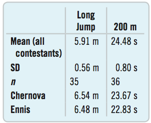
\[z = \frac{6.54 - 5.91}{0.56} \approx 1.1\]
Ennis’s 200 m run
\[z = \frac{22.83 - 24.48}{0.80} \approx -2.1\]
Ennis’s winning time is a little more impressive.
Judges could assign points based on standard deviations from mean and this system would have a correlation of 0.99 with the one currently used!
How Many Standard Deviations from Mean?
- \(-1 < z < 1\): Not uncommon
- \(z = \pm 3\): Rare
- \(z = 6\): Shouts out for attention!
National Health and Examination Survey
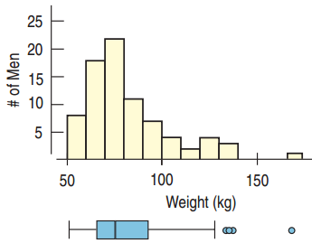
- Who? 80 male participants between 19 and 24 who measured between 68 and 70 inches tall
- What? Their weights in kilograms
- When? 2001 – 2002
- Where? United States
- Why? To study nutrition and health issues and trends
- How? National survey
Shifting Weights
Mean: 82.36 kg
Maximum Healthy Weight: 74 kg
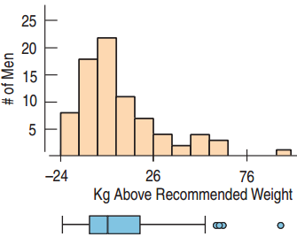
How are shape, center, and spread affected when 74 is subtracted from all values?
- Shape and spread are unaffected.
- Center is shifted by 74.
Rules for Shifting
If the same number is subtracted or added to all data values, then:
- The measures of the spread – standard deviation, range, and IQR – are all unaffected.
- The measures of position – mean, median, and mode – are all changed by that number.
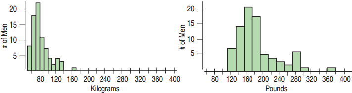
Rescaling
If we multiply all data values by the same number, what happens to the position and spread?
![]()
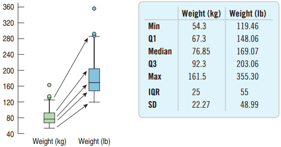
To go from kg to lbs, multiply by 2.2.
The mean and spread are also multiplied by 2.2.
How Rescaling Affects the Center and Spread
![]()
When we multiply (or divide) all the data values by a constant, all measures of position and all measures of spread are multiplied (or divided) by that same constant.
Example: Rescaling Combined Times in the Olympics
The mean and standard deviation in the men’s combined event at the Olympics were 168.93 seconds and 2.90 seconds, respectively.
If the times are measured in minutes, what will be the new mean and standard deviation?
- Mean: 168.93 / 60 = 2.816 minutes
- Standard Deviation: 2.90 / 60 = 0.048 minute
Shifting, Scaling, and z-Scores
Converting to z-scores:
\[z = \frac{y - \bar{y}}{s}\]
- Subtract the mean: \(\bar{y} - \bar{y} = 0\)
- Divide by the standard deviation: \(s / s = 1\)
Example: SAT and ACT Scores
How high does a college-bound senior need to score on the ACT in order to make it into the top quarter of equivalent of SAT scores for a college with middle 50% between 1530 and 1850?
- SAT: Mean = 1500, Standard Deviation = 250
- ACT: Mean = 20.8, Standard Deviation = 4.8
Plan: Want ACT score for upper quarter. Have \(\bar{y}\) and \(s\)
Variables: Both are quantitative. Units are points.
Show → Mechanics: Standardize the Variable
It is known that the middle 50% of SAT scores are between 1530 and 1850, \(\bar{y} = 1500\), \(s = 250\)
The top quarter starts at 1850.
Find the z-score:
\[z = \frac{1850 - 1500}{250} = 1.40\]
For the ACT, 1.40 standard deviations above the mean:
\[20.8 + 1.40(4.8) = 27.52\]
Conclusion
To be in the top quarter of applicants for that specific college in terms of combined SAT scores, a college-bound senior would need to have an ACT score of at least 27.52.
Models
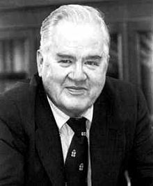
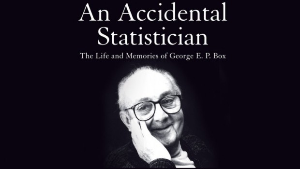
“All models are wrong, but some are useful.”
George Box, statistician
![]()
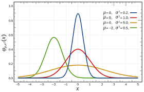
The Normal Model
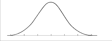
Bell Shaped: unimodal, symmetric
A Normal model for every mean and standard deviation.
- \(\mu\) (read “mew”) represents the population mean.
- \(\sigma\) (read “sigma”) represents the population standard deviation.
- \(N(\mu, \sigma)\) represents a Normal model with mean \(\mu\) and standard deviation \(\sigma\).
Parameters and Statistics
Parameters: Numbers that help specify the model
Statistics: Numbers that summarize the data
- \(\bar{y}\), \(s\), median, mode
\(N(0, 1)\) is called the standard Normal model, or the standard Normal distribution.
The Normal model should only be used if the data is approximately symmetric and unimodal.
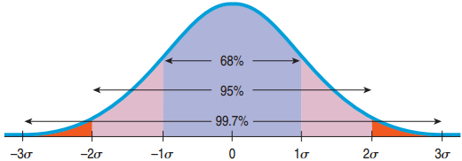
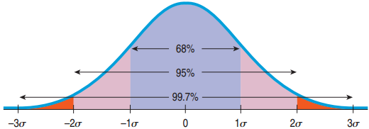
The 68-95-99.7 Rule
68% of the values fall within 1 standard deviation of the mean.
95% of the values fall within 2 standard deviations of the mean.
99.7% of the values fall within 3 standard deviations of the mean.
![]()
Example of the 68-95-99.7 Rule
In the 2010 winter Olympics men’s slalom, Li Lei’s time was 120.86 sec, about 1 standard deviation slower than the mean. Given the Normal model, how many of the 48 skiers were slower?
- About 68% are within 1 standard deviation of the mean.
- 100% – 68% = 32% are outside.
- “Slower” is just the left side.
- 32% / 2 = 16% are slower.
- 16% of 48 is 7.7.
- About 7 are slower than Li Lei.
Three Rules For Using the Normal Model
When data is provided, first make a histogram to make sure that the distribution is symmetric and unimodal.
Then sketch the Normal model.
Working With the 68-95-99.7 Rule
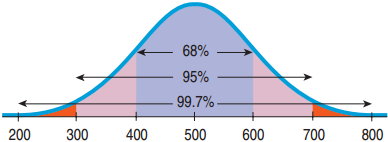
Each part of the SAT has a mean of 500 and a standard deviation of 100. Assume the data is symmetric and unimodal. If you earned a 600 on one part of the SAT how do you stand among all others who took the SAT?
- Plan: The variable is quantitative and the distribution is symmetric and unimodal. Use the Normal model \(N(500, 100)\).
Mechanics
Mechanics:
- Make a picture.
- 600 is 1 standard deviation above the mean.
Conclusion:
- 68% lies within 1 standard deviation of the mean.
- 100% - 68% = 32% are outside of 1 standard deviation of the mean.
- Above 1 standard deviation is half of that.
- Your score is higher than 84% of all scores on this test.
5.4
Finding Normal Percentiles
What if z is not −3, −2, −1, 0, 1, 2, or 3?
If the data value we are trying to find using the Normal model does not have such a nice z-score, we will use a table.
Example: Where do you stand if your SAT math score was 680? \(\mu = 500\), \(\sigma = 100\)
Note that the z-score is not an integer:
\[z = \frac{680 - 500}{100} = 1.8\]
The Z table
Look for the z-score on the table: 1.8
Look for the second decimal place.
Result: 0.9641
96.4% of SAT scores are below 680.
A Probability Involving “Between”
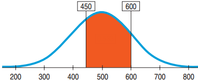
What is the proportion of SAT scores that fall between 450 and 600? \(\mu = 500\), \(\sigma = 100\)
Plan: Probability that \(x\) is between 450 and 600 = Probability that \(x < 600\) – Probability that \(x < 450\)
Variable: We are told that the Normal model works. \(N(500, 100)\)
A Probability Involving “Between”
What is the proportion of SAT scores that fall between 450 and 600? \(\mu = 500\), \(\sigma = 100\)
\[z = \frac{600 - 500}{100} = 1 \qquad z = \frac{450 - 500}{100} = -0.5\]
Probability that \(x\) is between 450 and 600
- = Probability that \(x < 600\) – Probability that \(x < 450\)
- = 0.8413 – 0.3085 = 0.5328
Conclusion: The Normal model estimates that about 53.28% of SAT scores fall between 450 and 600.
From Percentiles to Scores: z in Reverse
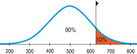
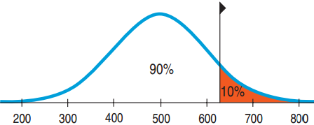
Suppose a college admits only people with SAT scores in the top 10%. How high a score does it take to be eligible? \(\mu = 500\), \(\sigma = 100\)
Plan: We are given the probability and want to go backwards to find \(x\).
Variable: \(N(500, 100)\)
From Percentiles to Scores: z in Reverse
Suppose a college admits only people with SAT scores in the top 10%. How high a score does it take to be eligible? \(\mu = 500\), \(\sigma = 100\)
\(z = 1.29\)
\[\frac{x - 500}{100} = 1.29\]
\[x = 1.29 \times 100 + 500 = 629\]
Conclusion: Because the school wants the SAT Verbal scores in the top 10%, the cutoff is 629.
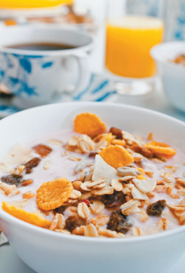
Underweight Cereal Boxes
Based on experience, a manufacturer makes cereal boxes that fit the Normal model with mean 16.3 ounces and standard deviation 0.2 ounces, but the label reads 16.0 ounces. What fraction will be underweight?
- Plan: Find Probability that \(x < 16.0\)
- Variable: \(N(16.3, 0.2)\)
Underweight Cereal Boxes
What fraction of the cereal boxes will be underweight (less than 16.0)? \(\mu = 16.3\), \(\sigma = 0.2\)
\[z = \frac{16.0 - 16.3}{0.2} = -1.5\]
Probability \(x < 16.0\) = 0.0668
Conclusion: I estimate that approximately 6.7% of the boxes will contain less than 16.0 ounces of cereal.
Underweight Cereal Boxes Part II
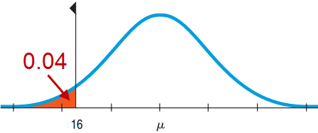
Lawyers say that 6.7% is too high and recommend that at most 4% be underweight. What should they set the mean at? \(\sigma = 0.2\)
Mechanics: Sketch a picture.
\(z = -1.75\)
Find \(16 + 1.75(0.2) = 16.35\) ounces
Conclusion: The company must set the machine to average 16.35 ounces per box.
Underweight Cereal Boxes Part III
The CEO vetoes that plan and sticks with a mean of 16.2 ounces and 4% weighing under 16.0 ounces. She demands a machine with a lower standard deviation. What standard deviation must the machine achieve?
- Plan: Find \(\sigma\) such that Probability \(x < 16.0 = 0.04\).
- Variable: \(N(16.2, ?)\)
Underweight Cereal Boxes Part III
What standard deviation must the machine achieve? \(N(16.2, ?)\)
From before, \(z = -1.75\)
\[-1.75 = \frac{16.0 - 16.2}{\sigma}\]
\[1.75\sigma = 0.2, \quad \sigma = 0.114\]
Conclusion: The company must get the machine to box cereal with a standard deviation of no more than 0.114 ounces. The machine must be more consistent.
5.5
Normal Probability Plots
Checking if the Normal Model Applies
A histogram will work, but there is an alternative method.
Instead use a Normal Probability Plot.
- Plots each value against the z-score that would be expected had the distribution been perfectly normal.
- If the plot shows a line or is nearly straight, then the Normal model works.
- If the plot strays from being a line, then the Normal model is not a good model.
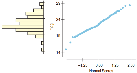
The Normal Model Applies
![]()
The Normal probability plot is nearly straight, so the Normal model applies. Note that the histogram is unimodal and somewhat symmetric.
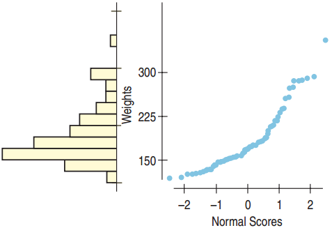
The Normal Model Does Not Apply
![]()
The Normal probability plot is not straight, so the Normal model does not apply. Note that the histogram is skewed right.
What Can Go Wrong
Don’t use the Normal model when the distribution is not unimodal and symmetric.
- Always look at the picture first.
Don’t use the mean and standard deviation when outliers are present.
- Check by making a picture.
Don’t round your results in the middle of the calculation.
- Always wait until the end to round.
Don’t worry about minor differences in results.
- Different rounding can produce slightly different results.