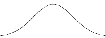
Quantitative Methods
Lecture 3
2020-07-08
Review
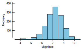
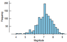
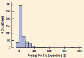
How to display quantitative data: histograms
- bin width
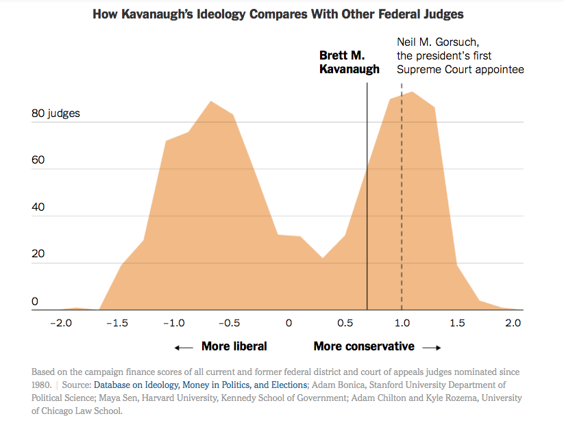
- shape: mode, symmetry, skew
- outliers
Review
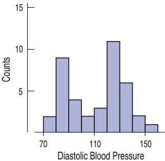
Example of bimodal distribution from The New York Times
Review
How to display quantitative data: histograms
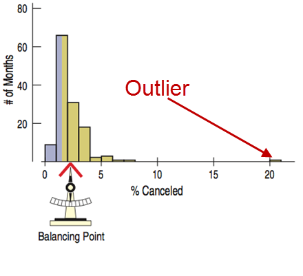
- CENTER: median, mean
- Median: the center of data values
- not sensitive to outliers
- Mean: average
- sensitive to outliers
\[\bar{y} = \frac{\sum y}{n}\]
- Mode: value that appears most often
Review
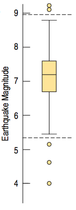
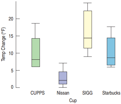
How to display quantitative data: boxplots
- SPREAD: range, IQR
- range: sensitive to outliers
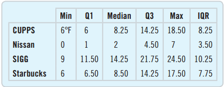
- five numbers summary
- IQR
- boxplot
Mechanics
Review
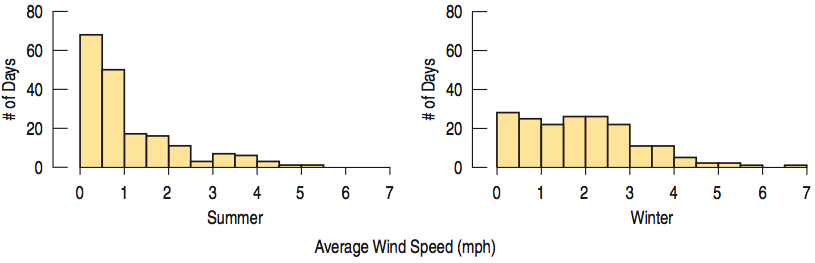
How to compare quantitative data: histograms and boxplots
Review
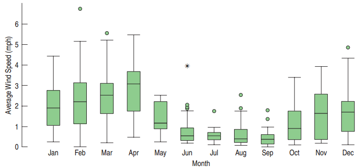
How to compare quantitative data: histograms and boxplots
Review: Timeplots
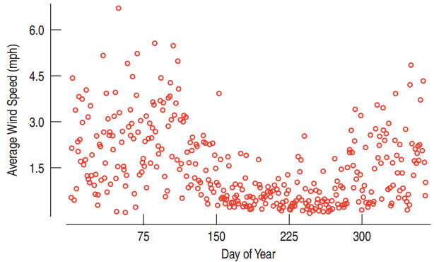
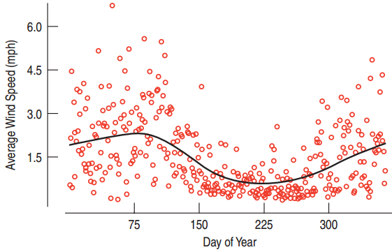
- Timeplots display every data value on a timeline.
- Great for spotting trends - easier with a lowess curve
- We can look into the future…
- …but we can never predict a single event, an extraordinary event or the stock market (random)
Review: Transformation of the Data
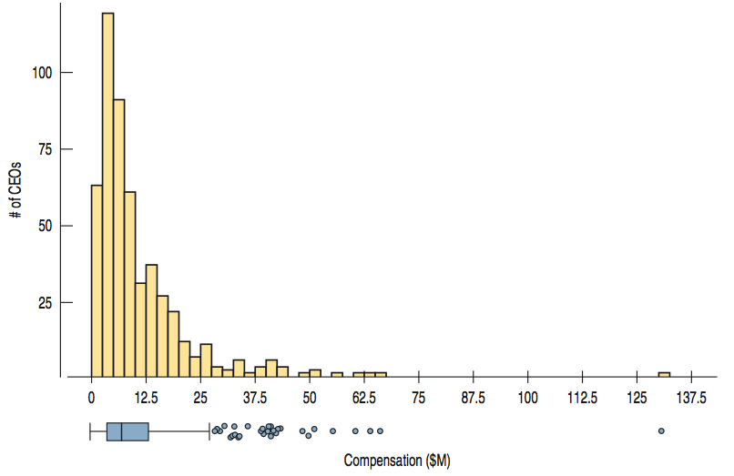
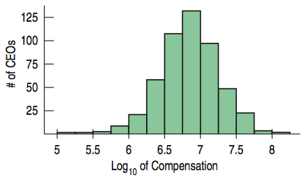
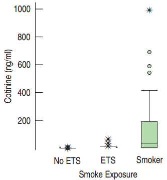
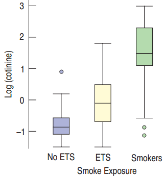
Taking the logarithm of the salaries makes the histogram much easier to interpret.
Apples and oranges

Comparing Athletes
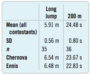
- Chernova took the gold in the 2012 Olympics with a long jump of 6.545 m
- About 0.5 m farther than the mean distance.
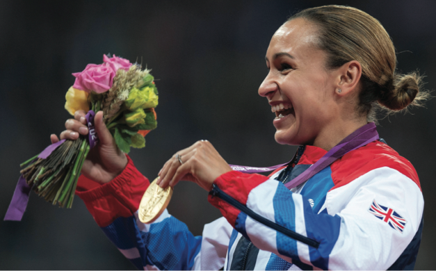
- Jessica Ennis won the 200 m run with a time of 22.83 s
- More than 2 s faster than average.
- Whose performance was more impressive?
How Many Standard Deviations Above?
The standard deviation helps us compare.
- Is there an even more precise way to calculate these?
- We can use a “z-score”
How Many Standard Deviations from Mean?
How Many Standard Deviations from Mean?
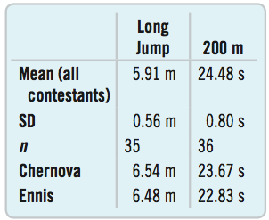
Chernova’s long jump
\[z = \frac{6.54 - 5.91}{0.56} \approx 1.1\]
Ennis’s 200 m run
\[z = \frac{22.83 - 24.48}{0.80} \approx -2.1\]
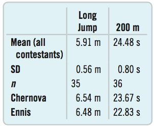
- Ennis’s winning time is a little more impressive.
- Judges could assign points based on standard deviations from mean and this system would have a correlation of 0.99 with the one currently used!
Shifting the Distribution
- Mean: 82.36 kg
- Maximum Healthy Weight: 74 kg
- How are shape, center, and spread affected when 74 is subtracted from all values?
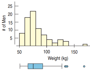
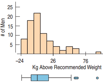
- Shape and spread are unaffected.
- Center is shifted by 74.
Rescaling
If we multiply all data values by the same number, what happens to the position and spread?
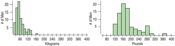
- To go from kg to lbs, multiply by 2.2.
- The mean and spread are also multiplied by 2.2.
- And how about the shape?
How Rescaling Affects the Center and Spread
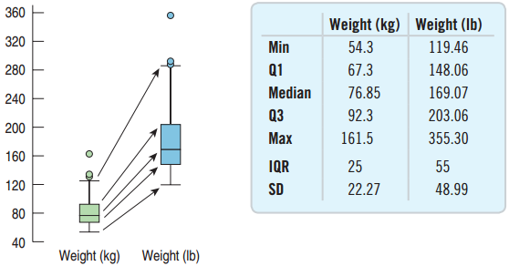
When we multiply (or divide) all the data values by a constant, all measures of position and all measures of spread are multiplied (or divided) by that same constant.
Models
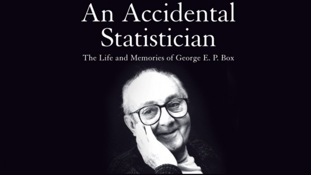
“All models are wrong, but some are useful.” – George Box, statistician
Review
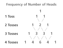
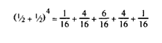
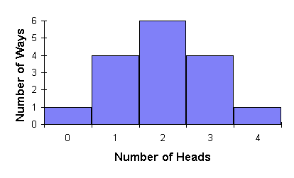
From the binomial expansion to the normal distribution
We can plot the frequency of getting heads on a histogram
Review
From the binomial expansion to the normal distribution
We can plot the frequency of getting heads on a histogram
Review
From the binomial expansion to the normal distribution
The more coin tosses I make, the more this histogram will resemble a curve:
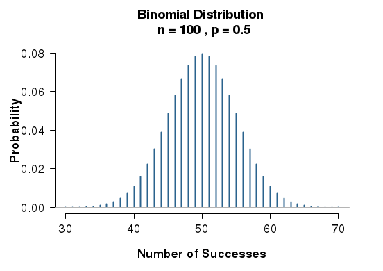
See simulation at: https://shiny.rit.albany.edu/stat/binomial/
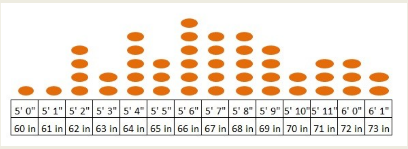
Students’ heights!
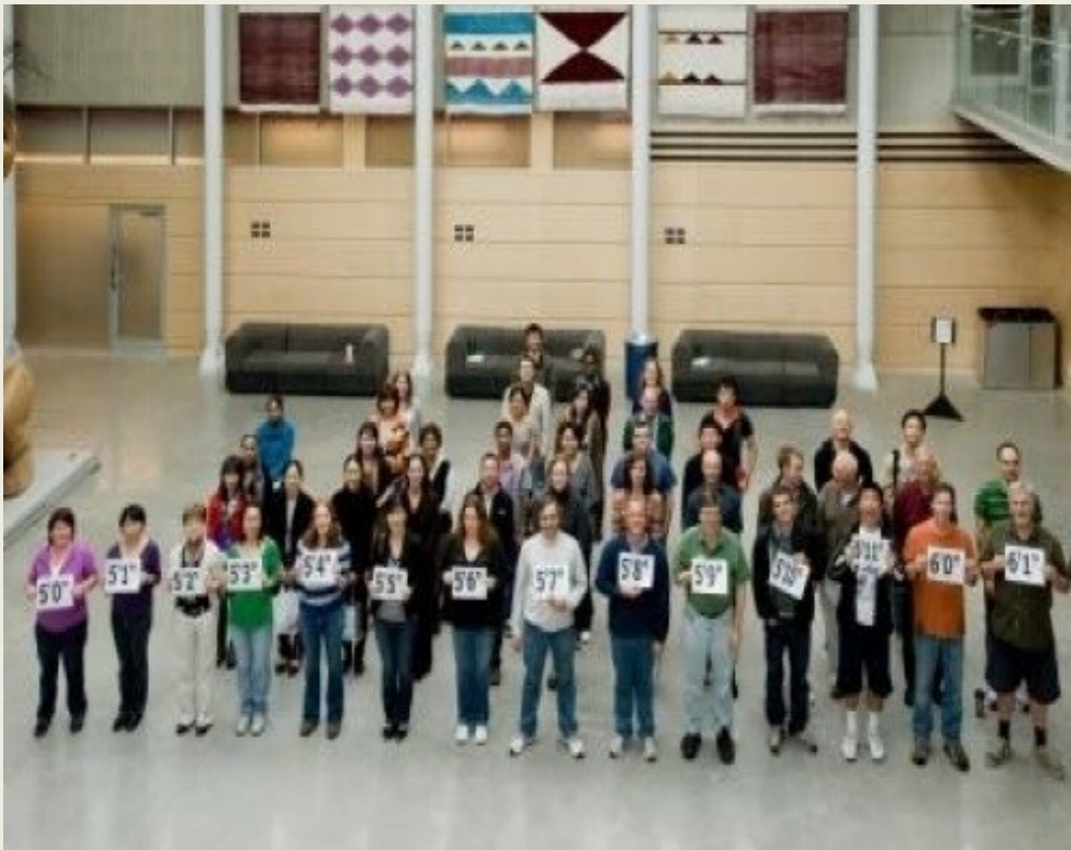
Students’ heights!
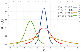
The Normal Model
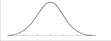
- Bell Shaped: unimodal, symmetric
- A Normal model for every value of mean and standard deviation.
- \(\mu\) (read “mew”) represents the population mean.
- \(\sigma\) (read “sigma”) represents the population standard deviation.
- \(N(\mu, \sigma)\) represents a Normal model with mean \(\mu\) and standard deviation \(\sigma\).
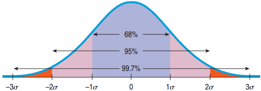
The 68-95-99.7 Rule
- 68% of the values fall within 1 standard deviation of the mean.
- 95% of the values fall within 2 standard deviations of the mean.
- 99.7% of the values fall within 3 standard deviations of the mean.
Probability is the area under the curve
Remember the binomial expansion? Let’s sketch it.
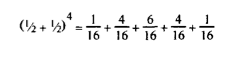
Probability as an area under the curve
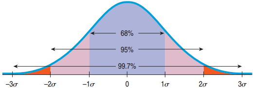
How Many Standard Deviations from Mean?
- \(-1 < z < 1\): Not uncommon
- \(z = \pm 3\): Rare
- \(z = 6\): Shouts out for attention!
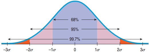
Example of the 68-95-99.7 Rule
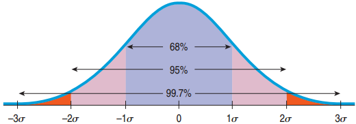
- In the 2010 winter Olympics men’s slalom, Li Lei’s time was 120.86 sec, about 1 standard deviation slower than the mean. Given the Normal model, how many of the 48 skiers were slower?
- About 68% are within 1 standard deviation of the mean.
- 100% - 68% = 32% are outside.
- “Slower” is just the left side.
- 32% / 2 = 16% are slower.
- 16% of 48 is 7.7.
- About 7 are slower than Li Lei.
Mechanics
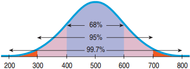
Mechanics:
- Make a picture.
Conclusion:
- 68% lies within 1 standard deviation of the mean.
- 100% - 68% = 32% are outside of 1 standard deviation of the mean.
- Above 1 standard deviation is half of that.
- 32% / 2 = 16%
- Your score is higher than 84% of all scores on this test.
Review: What if z is not -3, -2, -1, 0, 1, 2, or 3?
We will use a table. It gives you the percentile to the left
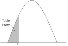
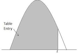
- Example: Where do you stand if your SAT math score was 680? \(\mu\) = 500, \(\sigma\) = 100
- Note that the z-score is not an integer:
\[z = \frac{680 - 500}{100} = 1.8\]
The Z table
- Look for the z-score on the table: 1.8
- Look for the second decimal place.
- Result: 0.9641
- 96.4% of SAT scores are below 680.
- Look for z-scores on the sides of the table, get percentage in the middle of the table
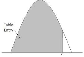
A Probability Involving “Between”
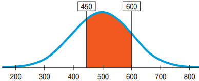
- What is the proportion of SAT scores that fall between 450 and 600? \(\mu\) = 500, \(\sigma\) = 100
- Plan: Probability that \(x\) is between 450 and 600 = Probability that \(x < 600\) \(-\) Probability that \(x < 450\)
- Variable: We are told that the Normal model works. \(N(500, 100)\)
From Percentiles to Scores: z in Reverse
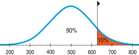
- Suppose a college admits only people with SAT scores in the top 10%. How high a score does it take to be eligible? \(\mu\) = 500, \(\sigma\) = 100
- Plan: We are given the probability and want to go backwards to find \(x\).
- Variable: \(N(500, 100)\)
From Percentiles to Scores: z in Reverse
- Suppose a college admits only people with SAT scores in the top 10%. How high a score does it take to be eligible? \(\mu\) = 500, \(\sigma\) = 100
- Look for percentage in middle of table, get z-score on the sides of it
- \(z = 1.29\)
- \((x - 500)/100 = 1.29\)
- \(x = 1.29 \cdot 100 + 500 = 629\)
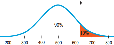
- Conclusion: Because the school wants the SAT Verbal scores in the top 10%, the cutoff is 629.
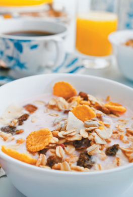
Quality control: Underweight Cereal Boxes
- Based on experience, a manufacturer makes cereal boxes that fit the Normal model with mean 16.3 ounces and standard deviation 0.2 ounces, but the label reads 16.0 ounces. What fraction will be underweight?
- Plan: Find Probability that \(x < 16.0\)
- Variable: \(N(16.3, 0.2)\)
Underweight Cereal Boxes Part II
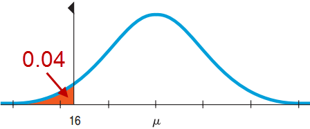
- Lawyers say that 6.7% is too high and recommend that at most 4% be underweight. What should they set the mean at? \(\sigma\) = 0.2
- Mechanics: Sketch a picture. What do we need?
- \(z = -1.75\)
- Find \(16 + 1.75(0.2) = 16.35\) ounces
- Conclusion: The company must set the machine to average 16.35 ounces per box.
The Normal Model Applies
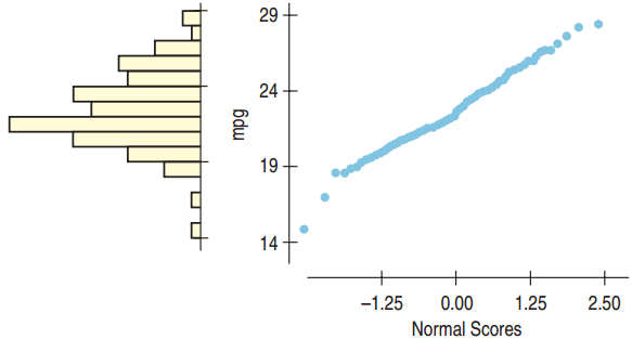
The Normal probability plot is nearly straight, so the Normal model applies. Note that the histogram is unimodal and somewhat symmetric.
The Normal Model Does Not Apply
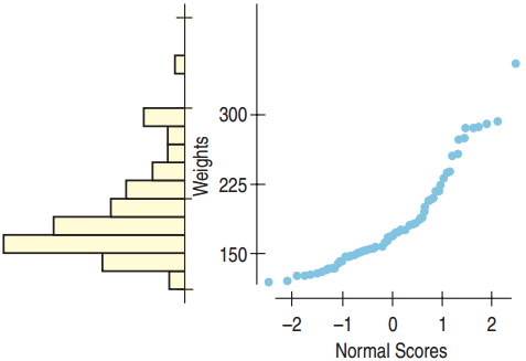
The Normal probability plot is not straight, so the Normal model does not apply. Note that the histogram is skewed right.
History of Statistics
- Demography
- Astronomy: how is measurement error distributed?
- Gambling: what are the odds of coin tosses?
- → study of binomial distribution
- → Gauss (1809) and Laplace (1812) find the equation of the Normal Distribution → the Law of Errors
- There was some variability in astronomy, but we solved it!