Quantitative Methods
Lecture 4
2020-07-09
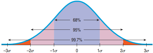
The 68-95-99.7 Rule
- 68% of the values fall within 1 standard deviation of the mean.
- 95% of the values fall within 2 standard deviations of the mean.
- 99.7% of the values fall within 3 standard deviations of the mean.
Example of the 68-95-99.7 Rule
In the 2010 winter Olympics men’s slalom, Li Lei’s time was 120.86 sec, about 1 standard deviation slower than the mean. Given the Normal model, how many of the 48 skiers were slower?
- About 68% are within 1 standard deviation of the mean.
- 100% − 68% = 32% are outside.
- “Slower” is just the right side.
- 32% / 2 = 16% are slower.
- 16% of 48 is 7.7.
- About 7 are slower than Li Lei.
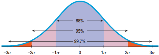
Review: What if z is not −3, −2, −1, 0, 1, 2, or 3?
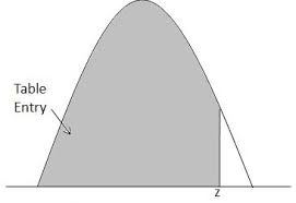
We will use a table. It gives you the percentile to the left.
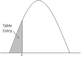
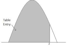
Example: Where do you stand if your SAT math score was 680? \(\mu = 500\), \(\sigma = 100\)
Note that the z-score is not an integer:
\[z = \frac{680 - 500}{100} = 1.8\]
The Z table
- Look for the z-score on the table: 1.8
- Look for the second decimal place.
- Result: 0.9641
- 96.4% of SAT scores are below 680.
A Probability Involving “Between”
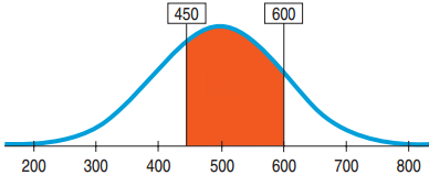
What is the proportion of SAT scores that fall between 450 and 600? \(\mu = 500\), \(\sigma = 100\)
- Plan: Probability that \(x\) is between 450 and 600 = Probability that \(x < 600\) − Probability that \(x < 450\)
- Variable: We are told that the Normal model works. \(N(500, 100)\)
From Percentiles to Scores: z in Reverse
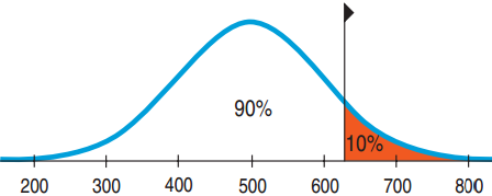
Suppose a college admits only people with SAT scores in the top 10%. How high a score does it take to be eligible? \(\mu = 500\), \(\sigma = 100\)
- Plan: We are given the probability and want to go backwards to find \(x\).
- Variable: \(N(500, 100)\)
From Percentiles to Scores: z in Reverse
Suppose a college admits only people with SAT scores in the top 10%. How high a score does it take to be eligible? \(\mu = 500\), \(\sigma = 100\)
- Look for percentage in middle of table, get z-score on the sides of it
- \(z = 1.29\)
- \((x - 500)/100 = 1.29\)
- \(x = 1.29 \times 100 + 500 = 629\)
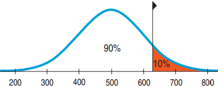
Conclusion: Because the school wants the SAT Verbal scores in the top 10%, the cutoff is 629.
Quality control: Underweight Cereal Boxes
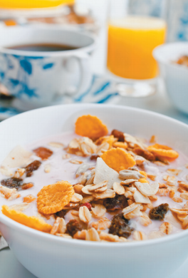
Based on experience, a manufacturer makes cereal boxes that fit the Normal model with mean 16.3 ounces and standard deviation 0.2 ounces, but the label reads 16.0 ounces. What fraction will be underweight?
- Plan: Find Probability that \(x < 16.0\)
- Variable: \(N(16.3, 0.2)\)
Underweight Cereal Boxes Part II
Lawyers say that 6.7% is too high and recommend that at most 4% be underweight. What should they set the mean at? \(\sigma = 0.2\)
- Mechanics: Sketch a picture. What do we need?
- \(z = -1.75\)
- Find \(16 + 1.75(0.2) = 16.35\) ounces
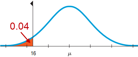
Conclusion: The company must set the machine to average 16.35 ounces per box.
The Normal Model Applies
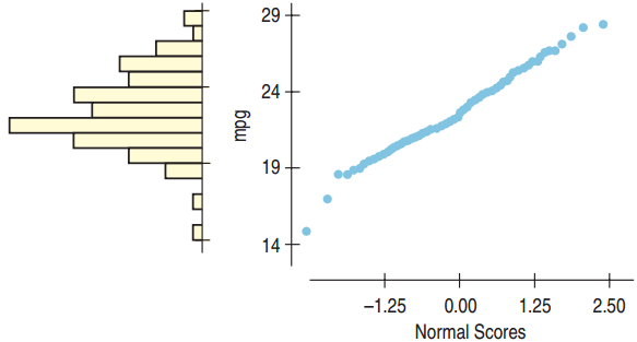
The Normal probability plot is nearly straight, so the Normal model applies. Note that the histogram is unimodal and somewhat symmetric.
The Normal Model Does Not Apply
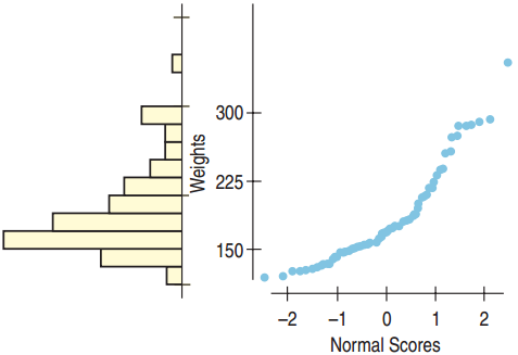
The Normal probability plot is not straight, so the Normal model does not apply. Note that the histogram is skewed right.
History of Statistics
Demography
Astronomy: how is measurement error distributed?
Gambling: what are the odds of coin tosses?
→ study of binomial distribution
→ Gauss (1809) and Laplace (1812) find the equation of the Normal Distribution → the Law of Errors
There was some variability in astronomy, but we solved it!
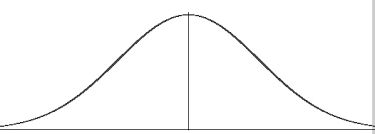
History of Statistics: Galton
- Sir Francis Galton (1822 – 1911)
- Darwin’s half cousin
- Studied variability and hereditary traits
- Problem: how to compare different features? → by their variation
- Idea: features that vary together are “co-related”
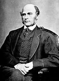
Galton
Law of error
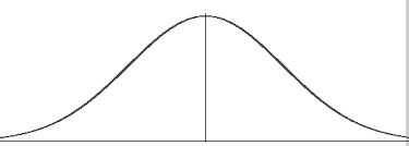
“I know of scarcely anything so apt to impress the imagination as the wonderful form of cosmic order expressed by the law of frequency of error. The law would have been personified by the Greeks if they had known of it. It reigns with serenity and complete self-effacement amidst the wildest confusion. The larger the mob, the greater the apparent anarchy, the more perfect is its sway. It is the supreme law of unreason.” (1889)
History of Statistics: Pearson
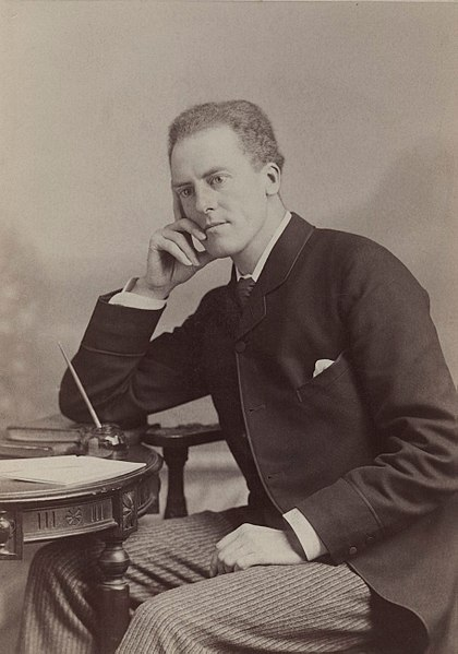
- Karl Pearson (1857 – 1936)
- Galton’s student
- Studied correlation in the context of variability and hereditary traits
- Came up with the correlation coefficient
The Direction of the Association
Negative Direction: As one goes up, the other goes down.

Positive Direction: As one goes up, the other goes up also.

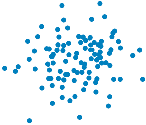
No Direction:
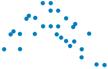
Form
Linear: The points cluster near a straight line.

Gently curves in a direction. May be able to straighten with a transformation.
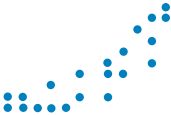
Curves up and down. Difficult to straighten
Strength of the Relationship
Strong Linear Relationship:
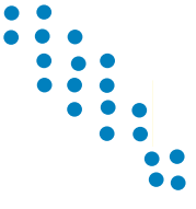
Moderate Linear Relationship:

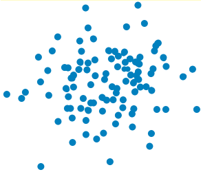
No Linear Relationship:
Outliers
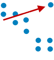
- An outlier is a point on a scatterplot that stands away from the overall pattern of the scatterplot.
- Outliers are almost always interesting and always deserve special attention.
Height and Weight
- How strong is the association between height and weight?
- It looks positive. How do we measure it?
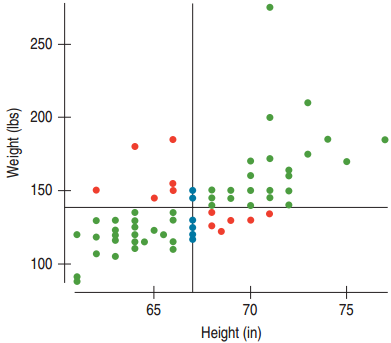
Positive association means: below/above average height predicts below/above average weight…
Green → +, Red → −, Blue → No Association
Correlation
- For the green dots: z-scores have the same sign, so multiplying the z-scores produces a positive value.
- For the red dots: z-scores have opposite signs, so multiplying the z-scores produces a negative value.
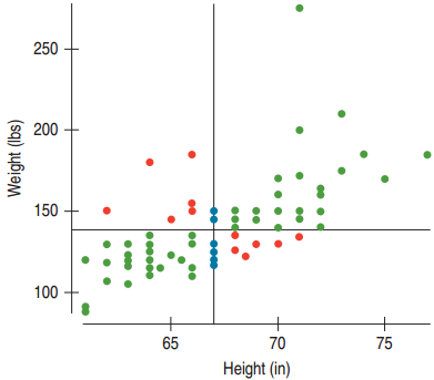
Define the correlation coefficient by an almost average product of the z-scores:
\[r = \frac{\sum z_x z_y}{n - 1}\]
Example: Clothes and Food Revisited
The scatterplot indicates a straight-line pattern. The variables are both quantitative ($), and there are no strong outliers away from the linear pattern.
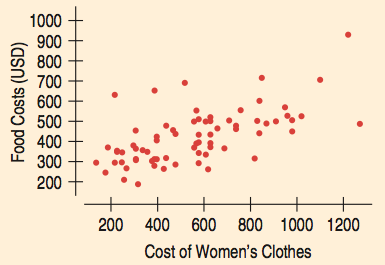
The correlation of \(r = 0.614\) represents a strong positive association.
Example: Vacation and Food Revisited
The scatterplot indicates that there may be no underlying linear relationship between vacation days and food costs.
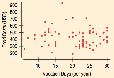
The correlation of \(r = -0.040\) supports that there may be no linear association between the two.
Blood Pressure Continued
Plot:
- Both variables are quantitative.
- The scatterplot is quite straight.
- There are no extreme outliers.
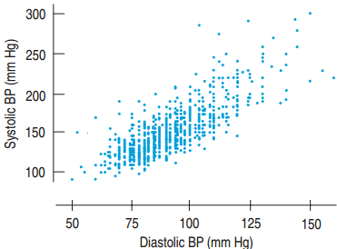
Therefore, correlation is a suitable measure of association.
Storks and Babies
There is a clear positive association between the number of storks and the population.
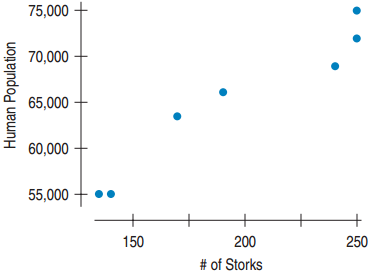
- This does not prove that an increase in storks has caused an increase in babies being born.
- Causation is in reverse. Storks nest on house chimneys, so the increased population has increased nesting sites.
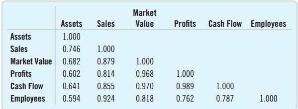
Correlation Tables
Often surveys or experiments contain many quantitative variables. A table can be used to show the correlation for each pair of variables.
Why do all the diagonals have 1.000?
Cautions about Correlation Tables
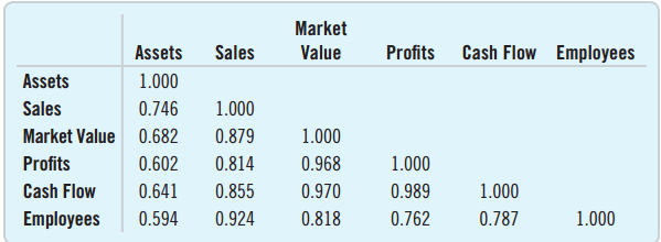
- Don’t blindly read a correlation table without first looking at each of the many scatterplots to check for linearity.
- You must also check for outliers.
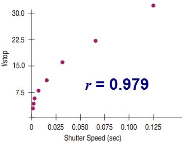
Shutter Speed and f/stop
- What’s wrong with concluding that since \(r = 0.979\) shutter speed and f/stop are strongly correlated?
- The scatter plot indicates that the two variables are not linearly related.
- Solution: Use a transformation, much like we did for histograms.
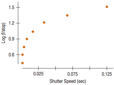
Re-expressing with log?
- How about the log transformation?
- This is even less linear!
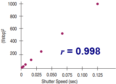
Re-Expressing
- The shutter speed and the square of the f/stop are linearly related.
- Now we can conclude that there is a very strong correlation between shutter speed and the square of the f/stop.
What Can Go Wrong?
- Make sure the association is linear.
- Always look at the scatterplot to check.
- Don’t assume the association is linear just because the correlation coefficient is high.
- Always look at the scatterplot to check.
- Beware of outliers!
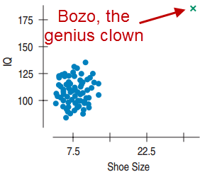
- \(r = 0.5\), but there is no correlation between shoe size and IQ.