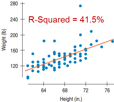
How strong is the association between height and weight?
It looks positive. How do we measure it?
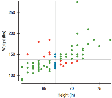
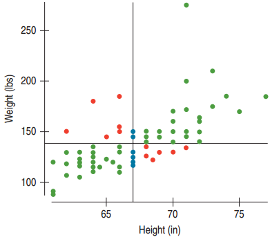
Positive association means above average height predicts above average weight.
Green → +, Red → -, Blue → No Association
Correlation
For the green dots: z-scores have the same sign, so multiplying the z-scores produces a positive value.
For the red dots: z-scores have opposite signs, so multiplying the z-scores produces a negative value.
Define the correlation coefficient by an almost average product of the z-scores:
\[r = \frac{\sum z_x z_y}{n-1}\]
Assumptions and Conditions for Correlation
To use r, there must be a true underlying linear relationship between the two variables.
The variables must be quantitative.
The pattern for the points of the scatterplot must be reasonably straight.
Outliers can strongly affect the correlation. Look at the scatterplot to make sure that there are no strong outliers.
Chapter 7
Linear Regression
7.1
Least Squares: The Line of “Best Fit”
The Linear Model
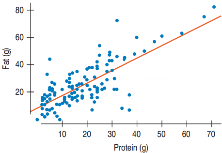
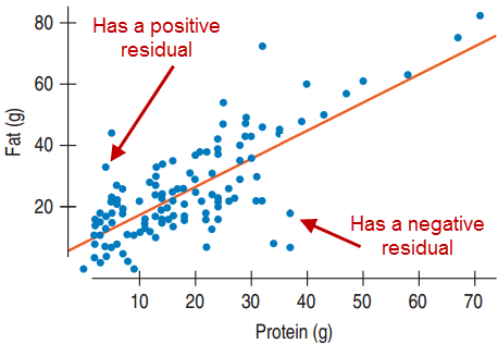
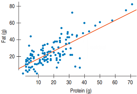
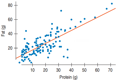
Fat and Protein at Burger King
The correlation is 0.76.
This indicates a strong linear fit, but how do we choose the line?
The line should be “closest” to the points.
How do we find it?
The Residual
\(\hat{y}\) is the value on the line
It is called the predicted value.
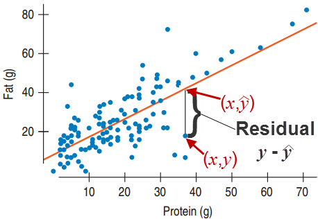
For each point \((x, y)\) look at the point \((x, \hat{y})\) on the line with the same x-coordinate.
The residual is defined by \(y - \hat{y}\)
The residual is the difference between the observed value and the predicted value.
More on Residuals
Residual:
Observed – Predicted
Points above the line have positive residuals
Points below the line have negative residuals.
This line gives the average fat content expected for a given amount of protein.
The Line of Best Fit
The best fitting line will have small residuals.
High negative residuals are just as “bad” as high positive residuals.
Squaring all residuals makes them all positive.
The line of best fit is the line for which the sum of the squares of the residuals is the smallest, also called the least squares line.
7.2
The Linear Model
What’s the equation of the Line of Best Fit?
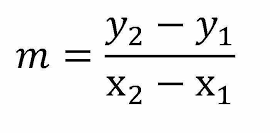
Line equation from Algebra
\(y = b + mx\)
Line of Best Fit
\(\hat{y} = b_0 + b_1 x\)
\(b_1\) is the slope: how rapidly \(\hat{y}\) changes with respect to \(x\).
\(b_0\) is the y-intercept: The value of \(\hat{y}\) when \(x\) is 0.
Interpreting the Line of Best Fit
Protein and Fat
What’s the slope? What does it mean?
Slope = 0.91: A Burger King item with one more gram of protein is expected to have 0.91 additional grams of fat.
What’s the y-intercept? What does it mean?
y-intercept = 8.4: A Burger King item with no grams of protein is expected to have 8.4 grams of fat. In reality the two items with no protein also have no fat.
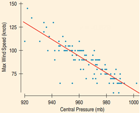
A Linear Model for Hurricanes
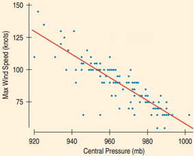
The barometric pressure at the center of a hurricane is often used to measure the strength of the hurricane because it can predict the maximum wind speed of the storm.
\(b_1\) = 0.76 × (16.2 gr fat / 13.5 gr protein) = 0.91 gr fat / gr prot
\(b_0\) = 24.8 − 0.91 gr fat / gr prot × 18.0 gr prot = 8.4 gr fat
Fat = 8.4 + 0.91 Protein
Conditions for Using Regression
The line of best fit is also called the least squares line or the regression line. Only use the regression line to make predictions if:
The variable must be Quantitative.
The relationship is Straight Enough.
There should be no strong Outliers.
Finally, always check if the prediction is reasonable.
7.4
Regression to the Mean
Correlation and Prediction, thinking in z-scores
A new male student joins the class. How tall is he in inches?
First guess would be the mean (\(\hat{z}_{in} = 0\)).
What if you also know his GPA was 3.9 (\(z_{GPA} = 2\))?
First guess would not change: the mean (\(\hat{z}_{in} = 0\))
If you were told his height in cm had \(z_{cm} = 2\)?
There is a perfect correlation between height in inches and height in cm
Now your guess would change, and you could find his height in inches exactly. (\(z_{in} = 2\))
Correlation and Prediction, thinking in z-scores
What would your guess for height be if you knew the student’s shoe size had \(z = 2\)?
We know that the correlation is positive, but not perfect (\(0 < z_{in} < 2\)).
There is a way to connect correlation and z-scores
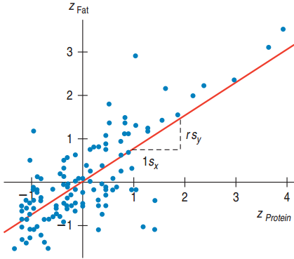
Let’s think about the line of best fit for z-scores
Since \(b_0 = \bar{y} - b_1\bar{x}\) and the means for z-scores are both 0, this gives \(b_0 = 0\).
Since the standard deviations are both 1, \(b_1 = r\frac{s_y}{s_x}\) gives \(b_1 = r\). Plugging into \(\hat{y} = b_0 + b_1 x\) gives:
\[\hat{z}_y = r z_x\]
Interpreting z-score Regression
If x is k standard deviations from its mean, then y will be r × k standard deviations from its mean.
Galton’s Discovery
Tall parents have tall children, but the children’s heights are likely to be closer to the mean than the parent’s heights.
Since \(-1 \leq r \leq 1\), \(rz_x\) is smaller in absolute value than the \(z_x\). This is called regression to the mean.
7.5
Examining the residuals
Residuals Revisited
The residual is the difference between the y value of the data point and the \(\hat{y}\) value found by plugging the x value into the least squares equation.
\[\text{Residual} = y - \hat{y}\]
To find the residual:
Plug x into the least squares equation to get \(\hat{y}\).
Subtract what you get from y to produce the residual.
Residual Example
\[\text{Residual} = y - \hat{y}\]
The data that compared central pressure and maximum wind speed had \(\hat{y} = 1024.464 - 0.968x\)
Hurricane Katrina’s central pressure was x = 920 millibars and the maximum wind speed was y = 150 knots (kts). What’s the residual?
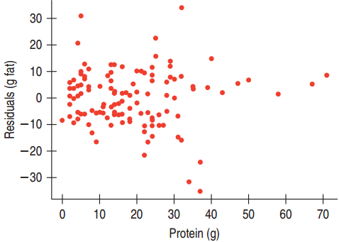
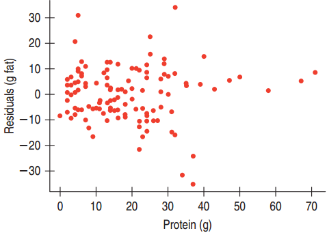
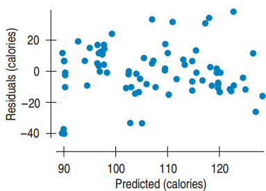
The regression model is a good model if the residual scatterplot against has no interesting features.
No direction
No shape
No bends
No outliers
No identifiable pattern
The Residual Standard Deviation
Since the mean of the residuals is 0, the standard deviation of the residuals is a measure of how small the residuals are.
Equal Variance Assumption: A good model will have the spread of the residuals consistent and small.
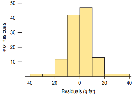
A histogram of the residuals helps us understand the residuals’ distribution.
7.6
R2 - The Variation Accounted for by the Model
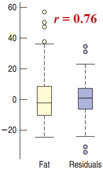
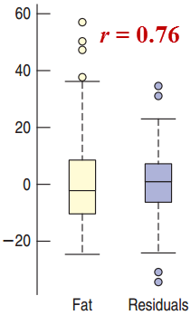
Comparing the Variation of y with the Variation of the Residuals
r = −1 or 1
The residuals are all 0. There is no variation of the residuals.
r = 0
The regression line is horizontal through the mean.
The residuals are the y values minus the mean.
The variation of the residuals would be the same as the variation of the original y values.
Comparing the Variation of y with the Variation of the Residuals: General r
The variation of the residuals for protein vs. fat for Burger King menu items is less than the variation for fat.
\(r^2\) (written \(R^2\)) gives the fraction of the data’s variation accounted for by the model.
Variation of y and the Variation of the Residuals (Continued)
\(R^2 = 0.76^2 = 0.58\)
58% of the variability in fat content in Burger King’s menu items is accounted for by the variation in the protein content.
42% of the variability in fat content is left in the residuals.
Other factors such as how the food is prepared account for this remaining variability.
R2 for Hurricanes
\(R^2\) = 0.803 for pressure and maximum wind speed
80.3% of the variability in maximum wind speeds of hurricanes is accounted for by the variation in pressure.
19.7% of the variability in maximum wind speeds is left in the residuals. Other factors such as temperature and location account for this remaining variability.
When is R2 Big Enough
\(R^2\) provides us with a measure of how useful the regression line is as a prediction tool.
If \(R^2\) is close to 1, then the regression line is useful.
If \(R^2\) is close to 0, then the regression line is not useful.
What “close to” means depends on who is using it.
Good Practice: Always report \(R^2\) and let the researcher decide.
Beware of Just Switching x and y
Switching x and y in the regression equation and solving for x does not give the equation of the regression line in reverse.
Instead, you must start over with all the computations.
This is no big deal if you use a computer or calculator, since the data is already entered.
7.7
Regression Assumptions and Conditions
Conditions to Check For
Quantitative Variable Condition: Regression analysis cannot be used for qualitative variables.
Straight Enough Condition: The scatterplot should indicate a relatively straight pattern.
Outlier Condition: Outliers dramatically influence the fit of the least squares line.
Does the Plot Thicken? Condition: The data should not become more spread out as the values of x increase. The spread should be relatively consistent for all x.
Conditions on the Scatterplot of the Residuals
There should be no bends.
There should be no outliers.
There should be no changes in the spread from one part of the plot to another.
Causation and Regression
Never report out a cause and effect relationship based solely on regression analysis.
Even though the correlation was high and the model was reasonably linear for pressure vs. wind in the hurricane data, we would need a scientific explanation to conclude cause and effect. Regression analysis alone can never prove cause and effect.
What Can Go Wrong?
Don’t fit a straight line to a nonlinear relationship.
If there are curves and bends in the scatterplot, don’t use regression analysis.
Don’t ignore outliers.
Instead report them out and think twice before using regression analysis.
Don’t invert the regression.
Switching x and y does not mean just solving for x in the least squares line. You must start over.
8.1
Examining Residuals
Chapter 8
Regression Wisdom
8.1
Examining Residuals
Why Examine the Residuals?
Looking at residuals is easiest way to check for linearity: the Straight Enough Condition
Residuals reveal subtleties not apparent from the scatterplot.
Residuals help us focus on the appropriateness of the regression line.
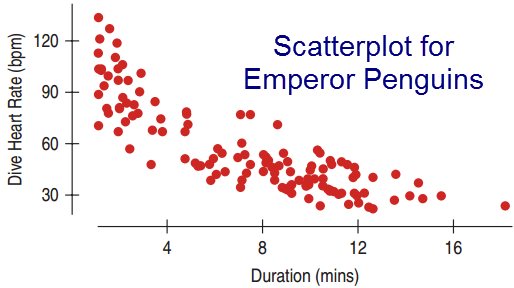
Without Looking at the Residuals
Analysis
\(R^2\) = 71.5%
Moderately strong negative association
\(\hat{y} = 96.9 - 5.47x\)
On average, for each minute the penguin is under water, its heart rate declines by 5.47 bpm.
The predicted heart rate before the dive is 96.9 bpm.
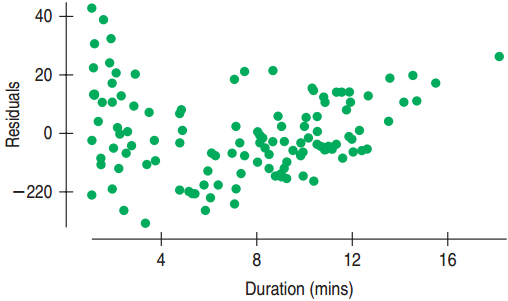
Examining the Residuals
What the Residuals Tell Us
There is a clear bend in the residual plot.
It is more spread out for low durations and less for high durations.
The residual plot suggests a re-expression may be needed to straighten out the data.
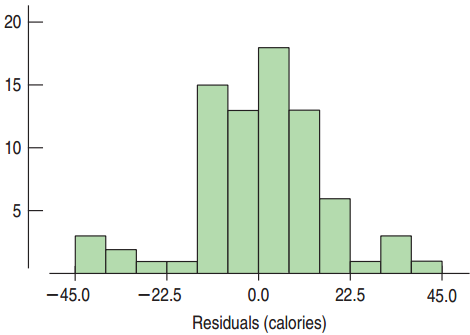
Examining the Histogram of the Residuals
What Does the Histogram Tell Us?
Close to Normal but:
Cluster of outliers on the left
Cluster of outliers on the right
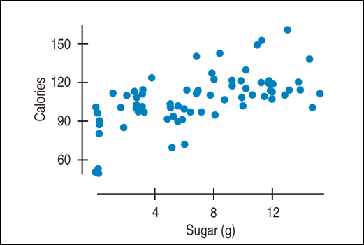
Cereals: sugar and calories
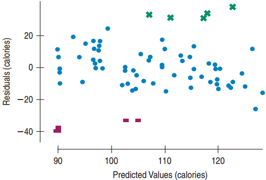
High Residual Cereals
Just Right Fruit & Nut
Muesli Raisins, Dates and Almonds
Mueslix Crispy Blend
Nutri-Grain Almond Raisin
All healthy cereals
It might be better to put healthy cereals in a separate group and analyze them separately.
Similarly, the lower group may need separating out.
Re-examining the Residual Plot
High Residual Cereals
Just Right Fruit & Nut
Muesli Raisins, Dates and Almonds
Mueslix Crispy Blend
Nutri-Grain Almond Raisin
All healthy cereals
It might be better to put healthy cereals in a separate group and analyze them separately.
Similarly, the lower group may need separating out.
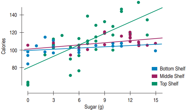
Subsets
This scatterplot shows the cereal boxes separated out by shelf: One line for each shelf.
8.2
Extrapolation: Reaching Beyond the Data
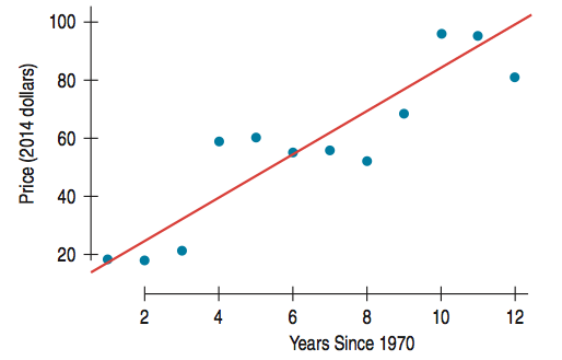
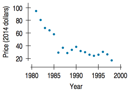
Predicting Gas Prices
\[\widehat{Price} = 12.79 + 6.75\ \text{Years Since 1970}\]
The data clearly follows a linear model.
Can we predict the price of oil for the year 25 (1995)?
\(12.79 + 6.75(25) \approx \$182\)
How good is this prediction?
How Well Did the Predictions Do?
Well, in the period from 1982 to 1998 oil prices didn’t exactly continue that steady increase. In fact, they went down so much that by 1998, prices (adjusted for inflation) were the lowest they’d been since before World War II.
Beware of Long Term Predictions
Actual vs. Predicted
Predicted for 1995: $182
Actual ≈ $25
What went wrong?
The regression line may not be a good predictor for values that are far from the collected data values, especially when x represents the date.
8.3
Outliers, Leverage and Influence
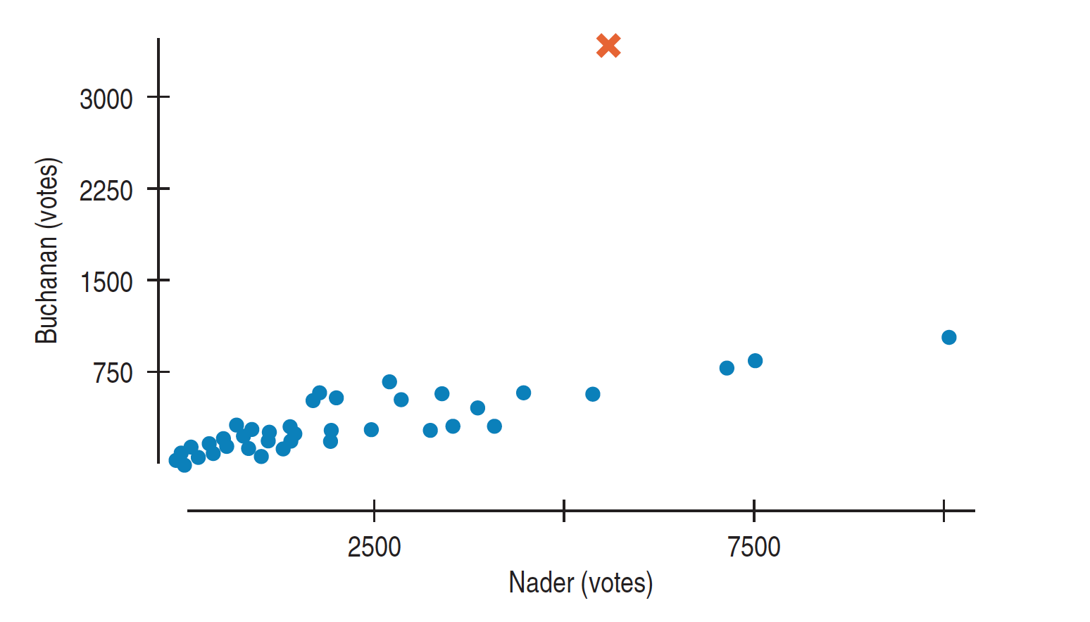
Leverage and Influential Points
A data point whose x-value is far from the mean of the rest of the x-values is said to have high leverage.
Leverage points have the potential to pull strongly on the regression line.
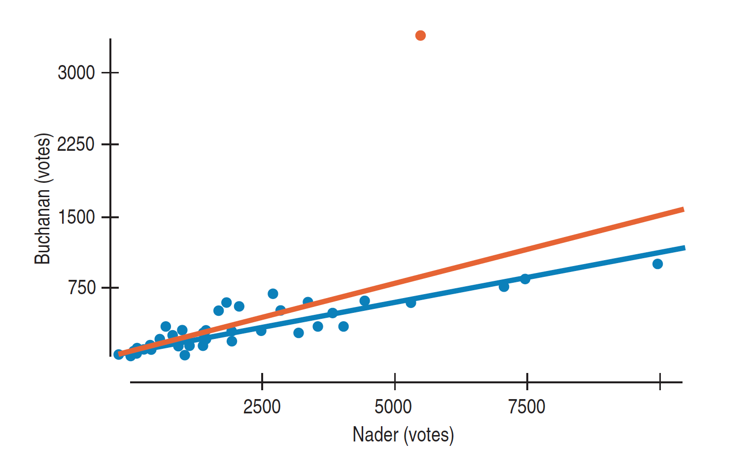
A point is influential if omitting it from the analysis changes the model enough to make a meaningful difference.
Influence is determined by
The residual
The leverage
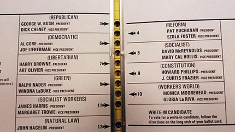
The 2000 elections and the Butterfly Ballot
The 2000 elections and the Butterfly Ballot
The 2000 elections and the Butterfly Ballot
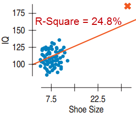
Shoe Size and IQ: Bozo the Genius Clown
Model that Includes Bozo
Almost all the variation accounted for by the model is from one point.
After removing the outlier \(R^2\) = 0.7%
Bozo is an influential point.
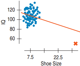
What if Bozo had an IQ of 50?
The slope would go from 0.96 IQ point/shoe size to \(-0.69\)
8.4
Lurking Variables and Causation
Two Examples of Regression
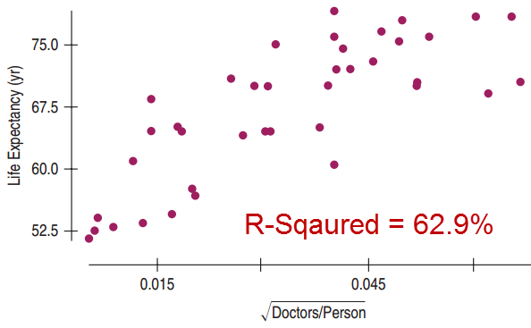
Doctors and Life Expectancy
There is a linear relationship between the square root of Doctors per person and Life Expectancy in 40 countries.
Should we send doctors to countries with low life expectancies?
Two Examples of Regression
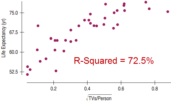
TV and Life Expectancy
There is a stronger linear relationship between the square root of TVs per person and Life Expectancy.
Should we send even more TVs to countries with low life expectancies?
Lurking Variables
Although both examples showed a positive linear relationship, this does not mean that if we send doctors or TVs to countries with low life expectancies, then their life expectancies will increase.
There could be a lurking variable such as standard of living.
Don’t confuse correlation with causation.
8.5
Working with Summary Values
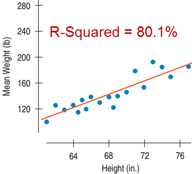
The Effect of Taking the Mean
Scatterplots of the mean show less variability.
Plotting the mean can give the false impression of a stronger correlation.
There is no standard correction for this.
What Can Go Wrong?
Make Sure the Relationship is Straight: Examine the residuals, especially the most extreme ones.
Look for Different Groups: Consider fitting a different linear model to each group.
Beware of Extrapolating: Don’t predict y-values for x-values that are far from the other x-values, especially when x represents time.
Look for Unusual Points: Use the scatterplot to find high leverage and influential points. Use a residual scatterplot to find large residual points.
What Can Go Wrong?
Beware of High Leverage Points, Especially Influential Points: Influential points can dominate.
Consider Comparing Two Regressions: Study the regression with and without the influential point.
Treat Unusual Points Honestly: Don’t just keep removing points until you are satisfied with the model. Just admit failure.
What Can Go Wrong?
Beware of Lurking Variables: A strong linear relationship does not mean that x causes y. Use good reasoning and science to determine the true cause. It may be a lurking variable.
Be Cautious of Summary Data: Statistics such as the mean and median tend to inflate the impression of the strength of the linear relationship.
Chapter 10
Understanding Randomness
10.1
What is Randomness?
1 2 3 4
Pick a number from 1 to 4
Is this random?
75% of all people pick 3.
How would you generate a random number?
We can use a computer or do it by hand.
In R there are different ways:
runif(1) generates one random # between 0 and 1
floor(runif(3, min=0, max=101)) generates 3 random integers between 0 and 100
Picking a Card
Randomness by Hand
Picking a card is another way to generate randomness.
Must shuffle at least 7 times to achieve randomness.
Other ways:
Rolling a die
Flipping a coin
Numbers out of a hat
10.2
Simulating by Hand
Lottery for the Dorms
57 students are in a lottery for the spacious triple dorm room. 20 were from the varsity team and all three winners were from this team.
How likely is this? Was it rigged?
Steps for Simulation
Specify how to model a component outcome using equally likely random digits:
Identify the component to be repeated.
Explain how you will model the experiment’s outcome.
Steps for Simulation
Specify how to simulate trials:
Explain how you will combine the components to model the trial.
State clearly what the response variable is.
Put it all together to run the simulation:
Run several (many) trials
Steps for Simulation
Analyze the response variable:
Collect and summarize the results of the trials.
As you have learned, look for shape, center, spread, outliers, etc.
State your conclusion
We estimate it takes a median of 5 boxes to complete the collection, but it could take a lot more.
Lottery for the Dorms
57 students are in a lottery for the spacious triple dorm room. 20 were from the varsity team and all three winners were from this team.
How likely is this? Was it rigged?
Plan → Simulation
Components to be repeated: Selection of the students.
Outcomes: Generate numbers from 1 to 57. 1-20 will represent the team members.
Only 3 out of the 100 trials resulted in “All Varsity.”
Conclusions
In the simulation, only 3 out of 100 were “All Varsity.”
While 3% is only a small chance, it is not impossible. It looks pretty suspicious.
Is 3% a small enough chance to make a formal accusation?
What Can Go Wrong?
Don’t Overstate Your Case
Simulation is not reality, it only indicates probability.
Model Outcome Chances Accurately
What would be wrong with generating random numbers 0, 1, 2, 3 to indicate the number of team members that room together?
There is not a 25% chance of each. They are not equally likely.
Run Enough Trials
Don’t just do a few trials. Err on the side of a large number of trials.
Chapter 11
Sample Surveys (11.1, 11.2, 11.3, 11.7)
11.1
The Three Big Ideas of Sampling
Idea 1: Examine a Part of the Whole
The Goal
Learn about the entire group of individuals (called the population)
The Problem
It is usually impossible to collect data on the entire population.
The Compromise
Collect data on a smaller group of individuals (called a sample) selected from the population.
Examples of Samples
People
Telephone surveys
Internet surveys
Data from a select group of customers
Student surveys handed out in class
Medical studies
Experimental units
Biological research
Crash dummy tests
Weather studies
Bias
The Challenge
Obtain a sample that is perfectly representative of the population.
Avoid bias – over or under emphasizing some characteristic of the population that is pertinent to the study.
Landon Beats Roosevelt??
The Survey
1936, Literary Digest received 2.4 million “mail in” ballots.
Used names from the phone book
The Results
Landon leads 57% to 43%
The Problem
Only high income earners could afford a phone.
This was a very biased survey.
Literary Digest soon went out of business.
Idea 2: Randomize
Can we list the characteristics of the population and ensure we represent them all without bias?
Race, age, ethnicity, income, marital status, work type, family size, …
The list would go on forever. There are more types of people than the number of people.
So… what can we do???
Randomizing can lead to a representative sample.
Randomizing protects us from the influences of all the features of the population.
On average, the sample will look like the population.
Idea 3: It’s the Sample Size
If you need 100 students to get a random sample at the university, how many Americans would you need to achieve the same level of randomness from the entire U.S.A.?
Answer: 100
It is the number of individuals, not the percent of individuals that matters.
The number of individuals in the sample is called the sample size.
Census
Why not just include everyone?
Surveying everyone is called a census.
That would be best if we could.
Problems with a census
Very expensive
Takes too long
Usually impossible to find everyone
Not everyone is willing to participate.
The population is always changing – births and deaths occur every day.
Issues with a Census
Double Counting
College students are often counted both at their colleges and where their parents live.
Under Counting: Who is likely to be missed?
The poor
Undocumented immigrants
Homeless
Should we use sampling instead of a census?
Statisticians think so.
Politicians don’t agree.
11.2
Populations and Parameters
Parameter and Statistic
Based on a study a report stated that 21.7% of all U.S. teens do not wear seatbelts.
Do they really know about all U.S. teens?
They used the sample proportion to make inferences about the population proportion.
A parameter is a number used in a model of the population.
A statistic is a number that is calculated from the sample data.
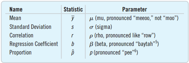
Greek for Parameter, Latin for Statistic
Examples of parameters
\(\mu\), \(\sigma\), \(p\), \(\rho\), \(\beta\)
Examples of Statistics
\(\bar{y}\), \(s\), \(\hat{p}\), \(r\), \(b\)
Notice that \(\pi\) would be confusing as a parameter.
Representative Sampling
Since we can’t take a true census, we want to compute statistics that reflect the parameters.
A sample that does the above is called a representative sample.
Biased samples tend to not be representative.
The statistic tends to be much higher or much lower than the parameter.
What’s Wrong with Each of the Following?
It is always better to take a census than draw a sample.
Stopping students outside of the cafeteria is a good way to find out about its quality of food.
To get the same level of precision that 100 students sampled from a university with 3000 students will have, you need to sample 1000 students from a university with 30,000 students.
What’s Wrong with Each of the Following?
The majority of the 12,357 students who answer a website poll clicked that they enjoyed doing statistics homework. Since the sample size is large, we can conclude that the majority of all students enjoy doing statistics homework.
The true percentage of all Statistics students who enjoy the homework is called a “population statistic.”
11.3
Simple Random Samples
Random But Not Representative
Random
Suppose there are 100 men and 100 women in a class. Flip a coin.
Heads: Choose the 100 men.
Tails: Choose the 100 women.
Every student has an equally likely chance of being chosen. Randomness was achieved.
This will not produce a representative sample.
Simple Random Sampling
SRS
Order the students from 1 to 40.
Use a computer to randomly select 20 numbers from 1 to 40.
Select the students with the chosen numbers.
Simple Random Sampling (SRS) is when every combination has an equally likely chance to be selected.
SRS is the standard by which all other sampling techniques are measured.
Statistical theory is based on SRS.
Sampling Variability
Samples will vary from one to the next.
The first sample of five students’ weight might average 131 pounds.
The second might average 138 pounds.
The sample to sample differences are called the sampling variability (or sampling error).
Natural
Not a problem
11.7
Common Sampling Mistakes, or How to Sample Badly
Mistake 1: Sample Volunteers
Voluntary Response Sample
Open the survey up to many, only a few respond.
Internet polls
Letters to Congress
“How are we doing?” cards
Sampling frame does not correspond to population.
Prone to bias
Only most opinionated respond.
Mistake 2: Sample Conveniently
In Convenience Sampling we sample only those who are convenient for us to sample.
Asking all of your Facebook friends.
Surveying at shopping malls to find how much people like shopping.
Asking people in a restaurant how often they eat out.
Convenience sampling is always biased.
More likely to get people like you.
“Safe-looking” people.
Mistake 3: Use a Bad Sampling Frame
Complete sampling frames are difficult. Missed are:
People in prison
Homeless people
Students
Long-term travelers
Cell-phone users who like their privacy
Mistake 4: Undercoverage
Bias can result when a subpopulation is left out or underrepresented.
Evening telephone surveys
Door-to-door surveys
Surveys given in English
Nonresponse Bias
Nonresponse bias is a concern for most surveys.
It is better to put forth effort to ensure a smaller group responds than to put the survey out to a large number and only receive a small number of responses.
Consider whether nonrespondents are likely to think differently from responders.
?
Response Bias
Response bias is anything in the survey design that influences the responses.
People want to please the interviewer.
People don’t want to admit they are flawed.
People hide personal facts: income, age, etc.
Wording of the question can steer the response.
How to Think about Bias
Always look for bias.
If there is bias in a survey that you have already conducted, you must start over. A larger sample size won’t help.