Quantitative Methods
Serena DeStefani – Lecture 7 – 7/15/2020
Lottery for the Dorms
57 students are in a lottery for the spacious triple dorm room. 20 were from the varsity team and all three winners were from this team.
- How likely is this? Was it rigged?
Conclusions
In the simulation, only 3 out of 100 were “All Varsity.”
While 3% is only a small chance, it is not impossible. It looks pretty suspicious.
Is 3% a small enough chance to make a formal accusation?
Idea 1: Examine a Part of the Whole
The Goal
- Learn about the entire group of individuals (called the population)
The Problem
- It is usually impossible to collect data on the entire population.
The Compromise
- Collect data on a smaller group of individuals (called a sample) selected from the population.
Bias
The Challenge
- Obtain a sample that is perfectly representative of the population.
- Avoid bias – over or under emphasizing some characteristic of the population that is pertinent to the study.
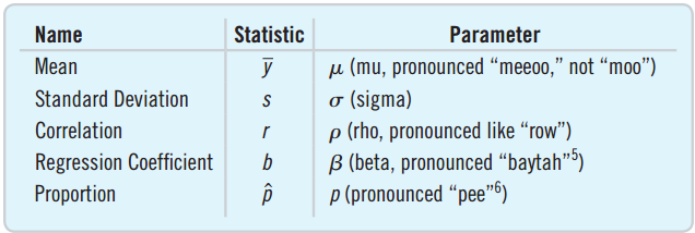
Greek for Parameter, Latin for Statistic
Examples of parameters
- \(\mu\), \(\sigma\), \(p\), \(\rho\), \(\beta\)
Examples of Statistics
- \(\bar{y}\), \(s\), \(\hat{p}\), \(r\), \(b\)
- Notice that \(\pi\) would be confusing as a parameter.
![]()
Idea 2: Randomize
Can we list the characteristics of the population and ensure we represent them all without bias?
- Race, age, ethnicity, income, marital status, work type, family size, …
- The list would go on forever. There are more types of people than the number of people.
- So… what can we do???
Randomizing can lead to a representative sample.
- Randomizing protects us from the influences of all the features of the population.
- On average, the sample will look like the population.
Idea 3: It’s the Sample Size
If you need 100 students to get a random sample at the university, how many Americans would you need to achieve the same level of randomness from the entire U.S.A.?
- Answer: 100
- It is the number of individuals, not the percent of individuals that matters.
- The number of individuals in the sample is called the sample size.
Simple Random Sampling
SRS
- Order the students from 1 to 40.
- Use a computer to randomly select 20 numbers from 1 to 40.
- Select the students with the chosen numbers.
Simple Random Sampling (SRS) is when every combination has an equally likely chance to be selected.
- SRS is the standard against which all other sampling techniques are measured.
- Statistical theory is based on SRS.
Sampling Variability
- Samples will vary from one to the next.
- The first sample of five students’ weight might average 131 pounds.
- The second might average 138 pounds.
The sample to sample differences are called the sampling variability (or sampling error).
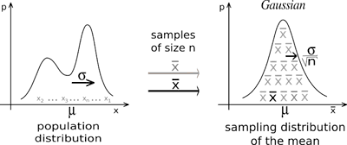
Central Limit Theorem
- As the number of samples increases, the distribution of the means of the samples becomes normal, regardless of the shape of the original population distribution
Classical Statistical Testing
- Why do we talk about:
- Simulation (the dorm lottery)
- Sampling
- Classical Statistical Testing is based on the idea of:
- running a study on a representative sample → results A
- “theoretically” repeating the study numerous times
- obtaining a theoretical probability distribution
- seeing how result A fares compared with this distribution
- It’s like running a simulation, except that we don’t do it
- Because of the Central Limit Theorem, we already know the distribution!
Chapter 13
From Randomness to Probability
Red Light, Green Light
Each day you drive through an intersection and check if the light is red, green, or yellow.
- Day 1: green
- Day 2: red
- Day 3: green
Before you begin, you know:
- An outcome will occur.
- The possible outcomes.
After you finish, you know:
- The outcomes that occurred
Random Phenomena Vocabulary
Trial
- Each occasion on which we observe a random phenomenon (the “thing” that is happening)
Outcome
- The value of the trial for the random phenomena (what could happen in a trial, specifically)
Event
- The combination of the trial’s outcomes (what actually happened)
Sample Space
- The collection of all possible outcomes (what could ever possibly happen)
Flipping Two Coins
Trial
- The flipping of the two coins
Outcome
- Heads or tails for each flip
Event
Sample Space
The Law of Large Numbers
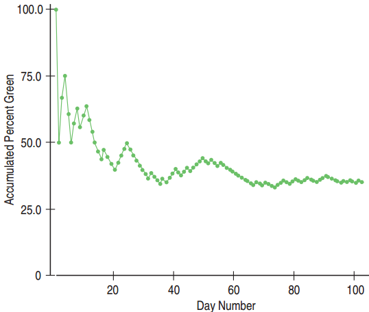
- If you flip a coin once, you will either get 100% heads or 0% heads.
- If you flip a coin 1000 times…
- …you will probably get close to 50% heads.
The Law of Large Numbers states that for many trials, the proportion of times an event occurs settles down to one number.
This number is called the empirical probability.
The Law of Large Numbers Requirements
Identical Probabilities
- The probabilities for each event must remain the same for each trial.
Independence
- The outcome of a trial is not influenced by the outcomes of the previous trials.
Empirical probability
- \(P(A) = \dfrac{\text{\# times A occurs}}{\text{\# of trials}}\) (in the long run)
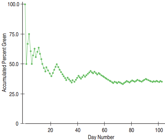
Red Light, Green Light: The Law of Large Numbers
- After many days, the proportion of green lights encountered is approximately 0.35.
- \(P(\text{green}) = 0.35\).
- If we recorded more days, the probability would still be about 0.35.
The Nonexistent Law of Averages
Wrong
- If you flip a coin 6 times and get 6 heads, then you are due for a tail on the next flip.
- You put 10 quarters in the slot machine and lose each time. You are just a bad luck person, so you have a smaller chance of winning on the 11th try.
- There is no such thing as the Law of Averages for short runs.
13.2
Modeling Probability
Theoretical Probability
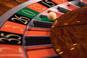
American Roulette
- 18 Red, 18 Black, 2 Green
- If you bet on Red, what is the probability of winning?
Theoretical Probability
- \(P(A) = \dfrac{\text{\# of outcomes in } A}{\text{\# of possible outcomes}}\)
- \(P(\text{red}) = \dfrac{18}{38}\)
Heads or Tails
Flip 2 coins. Find P(HH)
- List the sample space:
- \(P(\text{HH}) = \frac{1}{4}\)
Flip 100 coins. Find the probability of all heads.
- The sample space would involve 1,267,650,600,228,229,401,496,703,205,376 different outcomes.
- Later, we will see a better way.
Equally Likely?
What’s wrong with this logic?
- Randomly pick two people.
- Find the probability that both are left-handed.
- Sample Space: S = {LL, LR, RL, RR}
- \(P(\text{LL}) = \frac{1}{4}\)
Since left-handed and right-handed are not equally likely, this method does not work.
Personal Probability
What’s your chance of getting an A in a new course you are taking?
- You cannot base this on your long-run experience.
- There is no sample space of events with equal probabilities to list.
- You can only base your answer on subjective experience and guesswork.
- Probabilities based on personal experience rather than long-run relative frequencies or equally likely events are called personal probabilities.
Rules 1 and 2
Rule 1: \(0 \le P(A) \le 1\)
- You can’t have a −25% chance of winning.
- A 120% chance also makes no sense.
- Note: Probabilities are written in decimals.
- 45% chance → \(P(A) = 0.45\)
Rule 2: \(P(S) = 1\)
- The set of all possible outcomes has probability 1.
- There is a 100% chance that you will get a head or a tail.
Rule 3: The Complement Rule
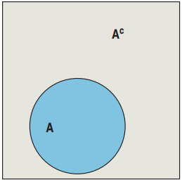
Complements
- Define \(A^C\) as the complement of \(A\).
- \(A^C\) is the event of “\(A\) not happening”.
- If \(A\) is the event of rolling a 5 on a six sided die, then \(A^C\) is the event of “not rolling a 5”: {1, 2, 3, 4, 6}
- \(P(A) = 1/6\). \(P(A^C) = ?\)
- \(P(A^C) = 5/6 = 1 - 1/6\)
The Rule of Complements: \(P(A^C) = 1 - P(A)\)
Red Light Green Light and Complements
We know that \(P(\text{green}) = 0.35\). Find \(P(\text{not green})\)
- Not green is the complement of green.
- Use the rule of complements:
\[\begin{align}
P(\text{not green}) &= P(\text{green}^C) \\
&= 1 - P(\text{green}) \\
&= 1 - 0.35 \\
&= 0.65
\end{align}\]
- The probability of the light not being green is 0.65.
Rule 4: The Addition Rule
Suppose \(P(\text{sophomore}) = 0.2\) and \(P(\text{junior}) = 0.3\)
- Find \(P(\text{sophomore OR junior})\)
- Solution: \(0.2 + 0.3 = 0.5\)
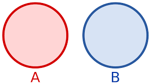
- This works because sophomore and junior are disjoint events. They have no outcomes in common.
The Addition Rule
- If \(A\) and \(B\) are disjoint events, then
- \(P(A \text{ OR } B) = P(A) + P(B)\)
Red Light, Green Light, Yellow Light
Given that \(P(\text{green}) = 0.35\) and \(P(\text{yellow}) = 0.04\)
- Find \(P(\text{red})\).
- Solution: Use the Rule of Complements and the Addition Rule.
\[\begin{align}
P(\text{red}) &= 1 - P(\text{red}^C) \\
&= 1 - P(\text{green OR yellow}) \\
&= 1 - [P(\text{green}) + P(\text{yellow})] \\
&= 1 - [0.35 + 0.04] = 1 - 0.39 \\
&= 0.61
\end{align}\]
The Sum of Probabilities
The sum of all the probabilities of every disjoint event must equal 1.
- What’s wrong with the following statement?
- Probabilities for freshmen, sophomore, junior, senior are: 0.25, 0.23, 0.22, 0.20.
- \(0.25 + 0.23 + 0.22 + 0.20 = 0.90\)
- Since they do not add to 1, something is wrong.
- How about the following?
- \(P(\text{owning a smartphone}) = 0.5\) and \(P(\text{owning a computer}) = 0.9\)
- This is fine, since they are not disjoint.
Rule 5: The Multiplication Rule
The probability that an Atlanta to Houston flight is on time is 0.85.
- If you have to fly every Monday, find the probability that your first two Monday flights will be on time.
Multiplication Rule: For independent events \(A\) and \(B\):
\[P(A \text{ AND } B) = P(A) \times P(B)\]
\[\begin{align}
P(\text{1st on time AND 2nd on time}) &= P(\text{1st on time}) \times P(\text{2nd on time}) \\
&= 0.85 \times 0.85 \\
&= 0.7225
\end{align}\]
Red Light AND Green Light AND Yellow Light
Find the probability that the light will be red on Monday, green on Tuesday, and yellow on Wednesday.
- The multiplication rule works for more than 2 events.
\[\begin{align}
&P(\text{red Mon. AND green Tues. AND yellow Wed.}) \\
&= P(\text{red Mon.}) \times P(\text{green Tues.}) \times P(\text{yellow Wed.}) \\
&= 0.61 \times 0.35 \times 0.04 \\
&= 0.00854
\end{align}\]
At Least One Red Light
Find the probability that the light will be red at least one time during the week.
\[\begin{align}
P(\text{at least 1 red}) &= 1 - P(\text{no reds}) \\
&= 1 - (0.39 \times 0.39 \times 0.39 \times 0.39 \times 0.39 \times 0.39 \times 0.39) \\
&\approx 0.9986
\end{align}\]
Japanese M&M Colors Desires: 38% Pink, 36% Teal, 16% Purple
- Find the probability that one Japanese survey respondent will want either pink or teal.
- Find the probability that two Japanese survey respondents will want purple.
- Find the probability that at least one of three Japanese survey respondents will want purple.
M&Ms: 38% Pink, 36% Teal, 16% Purple
- First notice that \(0.38 + 0.36 + 0.16 = 0.9 \ne 1\)
- There must be other colors.
Question: P(pink OR teal)
- Plan: Pink and teal are disjoint. Apply the Addition Rule.
M&Ms: 38% Pink, 36% Teal, 16% Purple
Question: P(pink OR teal)
\[\begin{align}
P(\text{pink OR teal}) &= P(\text{pink}) + P(\text{teal}) \\
&= 0.38 + 0.36 \\
&= 0.74
\end{align}\]
- Conclusion: The probability that the respondent chose pink or teal is 0.74.
M&Ms: 38% Pink, 36% Teal, 16% Purple
Question: P(1st purple AND 2nd purple)
- Plan: The choice made by the first respondent does not affect the choice of the other. The events are independent.
- Mechanics:
\[\begin{align}
P(\text{1st purple AND 2nd purple}) &= P(\text{1st purple}) \times P(\text{2nd purple}) \\
&= 0.16 \times 0.16 = 0.0256
\end{align}\]
- Conclusion: The probability that both choose purple is 0.0256.
M&Ms: 38% Pink, 36% Teal, 16% Purple
Question: P(at least 1 of 3 chose purple)
- Plan: Use the Rule of Complements and the Multiplication Rule. Note independence.
\[\begin{align}
P(\text{at least 1 of 3}) &= 1 - P([\text{at least 1 of 3}]^C) \\
&= 1 - P(\text{none of 3 chose purple}) \\
&= 1 - [P(\text{purple}^C)]^3
\end{align}\]
- \(P(\text{purple}^C) = 1 - P(\text{purple})\)
M&Ms: 38% Pink, 36% Teal, 16% Purple
Question: P(at least 1 of 3 chose purple)
\[\begin{align}
P(\text{at least 1 of 3 purple}) &= 1 - [P(\text{purple}^C)]^3 \\
&= 1 - [1 - 0.16]^3 \\
&= 1 - (0.84)^3 \\
&= 0.4073
\end{align}\]
- Conclusion: There’s about a 40.7% chance that at least one of the respondents chose purple.
What Can Go Wrong?
- Beware of probabilities that don’t add up to 1.
- If they add to less than 1, look for another category.
- If they add to more than 1, maybe they are not disjoint.
- Don’t add probabilities of events if they are not disjoint.
- Events must be disjoint to use the Addition Rule.
What Can Go Wrong?
- Don’t multiply probabilities of events if they are not independent.
- \(P(\text{over 6' and on basketball team})\) is not equal to \(P(\text{over 6'}) \times P(\text{on basketball team})\)
- Don’t confuse disjoint and independent
- Disjoint events are never independent.
Chapter 14
Probability Part 2
14.1
The General Addition Rule
Or But Not Disjoint
Your Wallet
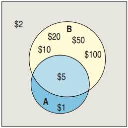
- S = {$1, $2, $5, $10, $20, $50, $100}
- A = {odd numbered value} = {$1, $5}
- B = {bill with a building} = {$5, $10, $20, $50, $100}
- Why is \(P(A \text{ or } B) \ne P(A) + P(B)\)?
- Answer: \(A\) and \(B\) are not disjoint.
- The intersection \(A\) and \(B\) = {$5} is double counted.
- To find \(P(A \text{ or } B)\), subtract \(P(A \text{ and } B)\).
The General Addition Rule
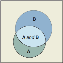
\[P(A \text{ or } B) = P(A) + P(B) - P(A \text{ and } B)\]
- The General Addition Rule in words: Add the probabilities of the two events and then subtract the probability of their intersection.
\(P(\text{odd amount or bill with a building})\)
\(= P(A) + P(B) - P(A \text{ and } B)\)
\(= P(\{\$1, \$5\}) + P(\{\$5, \$10, \$20, \$50, \$100\}) - P(\{\$5\})\)
General Addition Rule Example
Survey
- Are you currently in a relationship?
- Are you involved in sports?
Results
- 33% are in a relationship.
- 25% are involved in sports.
- 11% answered “yes” to both.
Problem
- Find the probability that a randomly selected student is in a relationship or is involved in sports.
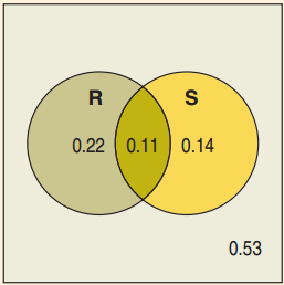
33% Relationship, 25% Sport, 11% Both
Events
- \(R\) = {in a relationship}
- \(S\) = {involved in sports}
Calculations
\[\begin{align}
P(R \text{ or } S) &= P(R) + P(S) - P(R \text{ and } S) \\
&= 0.33 + 0.25 - 0.11 \\
&= 0.47
\end{align}\]
Conclusion
- There is a 47% chance that a randomly selected student is in a relationship or is involved in sports.
Using Venn Diagrams
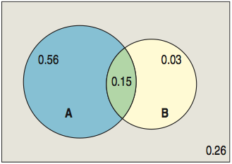
P(not in relationship and no sports)
- \(P(R^C \text{ and } S^C)\)
- This is the part outside of both circles: 0.53.
P(in a relationship but no sports)
- \(P(R \text{ and } S^C)\)
- This is the part in the circle \(R\) that is outside \(S\): 0.22.
P(in a relationship or involved in sports but not both)
- \(P((R \text{ and } S^C) \text{ or } (R^C \text{ and } S))\)
- This is the combination of the circles minus the intersection: \(0.22 + 0.14 = 0.36\)
14.2
Conditional Probability and the General Multiplication Rule
Contingency Table
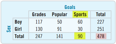
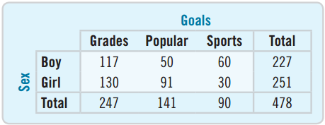
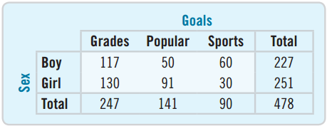
A table that displays the results of two categorical questions is called a contingency table.
- \(P(\text{girl}) = 251/478 = 0.525\)
- \(P(\text{girl and popular}) = 91/478 = 0.190\)
- \(P(\text{sports}) = 90/478 = 0.188\)
Conditional Probability
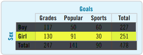
- What if we knew the chosen person was a girl? Would that change the probability that the girl’s goal was sports?
- Yes! We write \(P(\text{sports} \mid \text{girl})\)
- Only look at Girl row: \(P(\text{sports} \mid \text{girl}) = 30/251 = 0.120\)
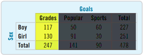
- Find the probability of selecting a boy given the goal is grades.
- \(P(\text{boy} \mid \text{grades}) = 117/247 = 0.474\)
College Students: Relationships and Sports
33% in relationships, 25% in sports, 11% in both
- If you see a student athlete, what is the probability that this athlete is in a relationship?
- \(P(R) = 0.33\), \(P(S) = 0.25\), \(P(R \text{ and } S) = 0.11\)
\[P(R \mid S) = \frac{P(R \text{ and } S)}{P(S)} = \frac{0.11}{0.25} = 0.44\]
- There is a 0.44 probability the student involved in sports is in a relationship. Notice this is higher than the probability for the general student (0.33).
The General Multiplication Rule
- For \(A\) and \(B\) independent, we had: \[P(A \text{ and } B) = P(A) \times P(B)\]
- Rearranging the conditional probability equation, we get the General Multiplication Rule: \[P(A \text{ and } B) = P(A) \times P(B \mid A)\]
- Equivalently, \[P(A \text{ and } B) = P(B) \times P(A \mid B)\]
Definition of Independence
- Events \(A\) and \(B\) are independent if knowing \(A\) happened does not change the probability of \(B\). In symbols:
\[A \text{ and } B \text{ are independent} \leftrightarrow P(B \mid A) = P(B)\]
- Equivalent formulas for independence:
- \(P(A \mid B) = P(A)\)
- \(P(A \text{ and } B) = P(A) \times P(B)\)
Grades and Girl Independent?
- Determine if the “goal of good grades” and gender are independent.
- \(P(\text{grades} \mid \text{girl}) = 130/251 \approx 0.52\)
- \(P(\text{grades}) = 247/478 \approx 0.52\)
- To two decimal places, they are independent.
- Are the “goal of sports” and gender independent?
- \(P(\text{sports} \mid \text{boy}) = 60/227 \approx 0.26\)
- \(P(\text{sports}) = 90/478 \approx 0.19\)
- No, the goal of sports and gender are dependent.
Relationships, Sports, and Independence
33% in a relationship, 25% involved in sports, 11% both
- Are being in a relationship and being involved in sports independent?
- \(P(\text{relationship}) = 0.33\)
- \(P(\text{sports}) = 0.25\)
- \(P(\text{relationship and sports}) = 0.11\)
- \(0.33 \times 0.25 = 0.0825 \ne 0.11\)
- No, they are dependent.
- Are they disjoint?
- \(P(\text{relationship and sports}) = 0.11 \ne 0\)
- No, they are not disjoint.
Independent ≠ Disjoint
Disjoint events cannot be independent.
- Consider the events:
- Course grade A
- Course grade B
- Disjoint: You can’t get both.
- Not independent: \(P(A \mid B) = 0 \ne P(A)\)
- A and B are disjoint (also called mutually exclusive) but not independent.
Independence and Insurance
An insurance company insures 1000 houses
- If each house is in a different location, then the destruction of each can be treated as independent.
- \(P(\text{many are destroyed this year})\) is very small.
- If they are all in the same location, then they can all be destroyed by the same disaster. The events are not independent.
- \(P(\text{many are destroyed this year})\) is not as small.
- The insurance company has less risk with the former.
14.4
Picturing Probability: Tables, Venn Diagrams, and Trees
Marginal and Joint Probabilities
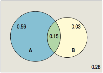
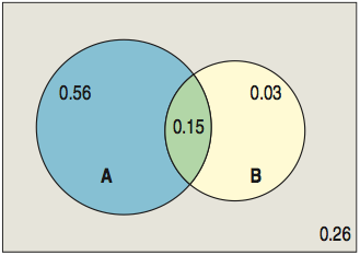
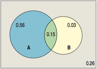
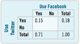
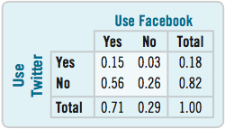
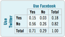
- 71% use Facebook, 18% Twitter, 15% both
- Draw a partial table.
- 0.71 and 0.18 are called marginal probabilities.
- 0.15 is a joint probability.
- How can we complete the table?
- The sum must add up
- \(0.15 + \; ? = 0.71\)
- \(0.18 + \; ? = 1.00\)