Review on Tuesday and Wednesday: please email questions/topic for review
Midterm on Thursday
Random Phenomena Vocabulary
Trial
Each occasion on which we observe a random phenomenon (the “thing” that is happening)
Outcome
The value of the trial for the random phenomenon (what could happen in a trial, specifically)
Event
The combination of the trial’s outcomes (what actually happened)
Sample Space
The collection of all possible outcomes (what could ever possibly happen)
Flipping Two Coins
Trial
The flipping of the two coins
Outcome
Heads or tails for each flip
Event
HT, for example
Sample Space
S = {HH, HT, TH, TT}
The Law of Large Numbers
If you flip a coin once, you will either get 100% heads or 0% heads.
If you flip a coin 1000 times…
…you will probably get close to 50% heads.
The Law of Large Numbers states that for many trials, the proportion of times an event occurs settles down to one number.
This number is called the empirical probability.
The Nonexistent Law of Averages
Wrong
If you flip a coin 6 times and get 6 heads, then you are due for a tail on the next flip.
You put 10 quarters in the slot machine and lose each time. You are just a bad luck person, so you have a smaller chance of winning on the 11th try.
There is no such thing as the Law of Averages for short runs.
Theoretical Probability
American Roulette
18 Red, 18 Black, 2 Green
If you bet on Red, what is the probability of winning?
Theoretical Probability
\[P(A) = \frac{\text{\# of outcomes in } A}{\text{\# of possible outcomes}}\]
\[P(\text{red}) = \frac{18}{38}\]
Rules: 1, 2 and 3
Rule 1: \(0 \le P(A) \le 1\)
That’s how we define probability
Rule 2: \(P(S) = 1\)
The set of all possible outcomes has probability 1
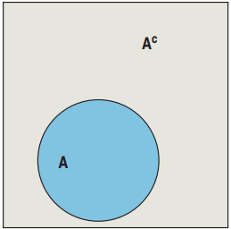
The Rule of Complements: \(P(A^C) = 1 - P(A)\)
\(A^C\) is the event of “A not happening”.
Events
Disjoint
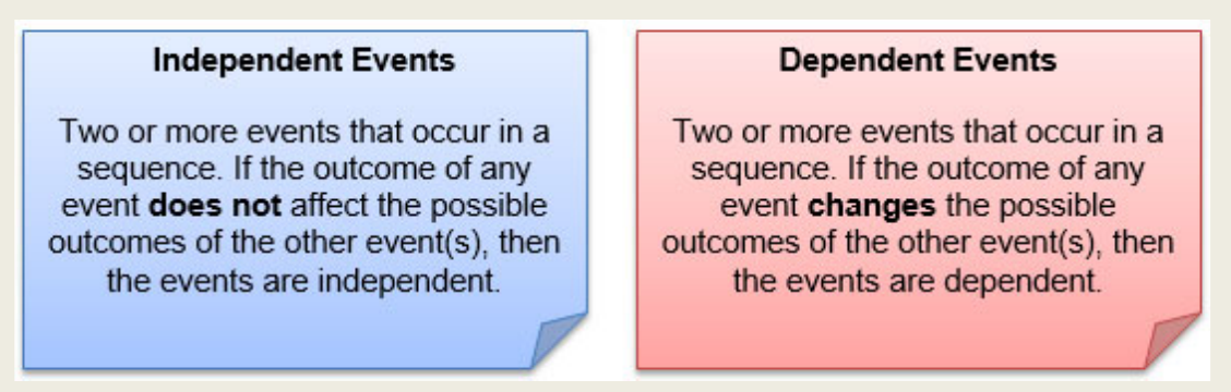
Independent and Dependent
Events
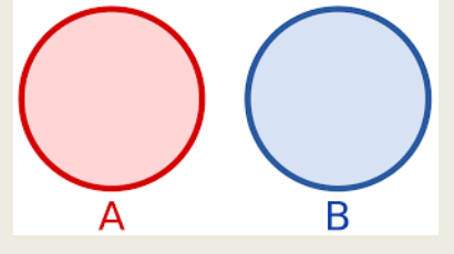
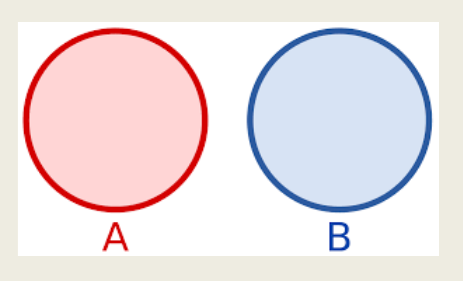
Disjoint events:
OR: Addition
AND: makes no sense
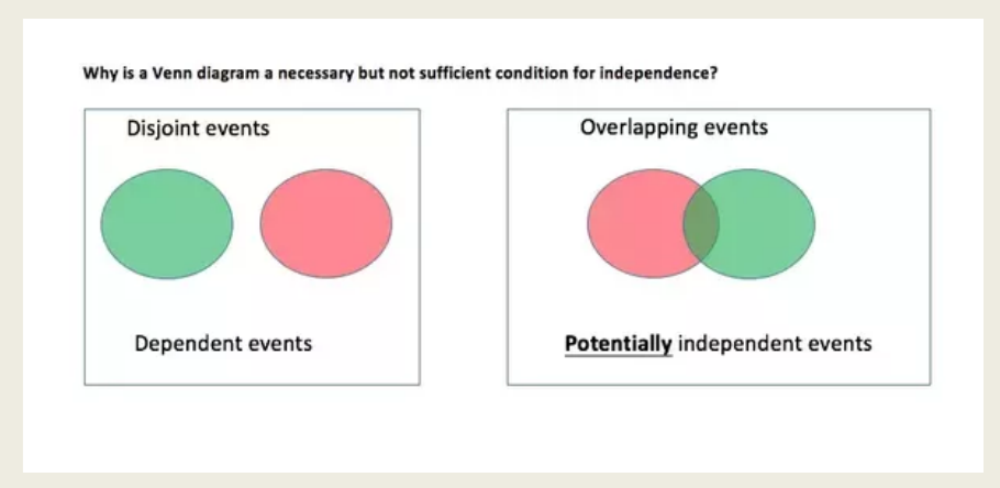
But what if two events overlap? They can be either independent or dependent
OR but not disjoint? General addition rule
AND?
If they are independent: Multiplication rule
If they are dependent, General Multiplication rule
Events
Disjoint
Overlapping
Dependent
YES
YES
Independent
DOES NOT EXIST
YES
Rule 4: The Addition Rule
Suppose \(P(\text{sophomore}) = 0.2\) and \(P(\text{junior}) = 0.3\)
Find \(P(\text{sophomore OR junior})\)
Solution: \(0.2 + 0.3 = 0.5\)
This works because sophomore and junior are disjoint events. They have no outcomes in common.
The Addition Rule
If A and B are disjoint events, then
\[P(A \text{ OR } B) = P(A) + P(B)\]
Rule 5: The Multiplication Rule
The probability that an Atlanta to Houston flight is on time is 0.85.
If you have to fly every Monday, find the probability that your first two Monday flights will be on time.
Multiplication Rule: For independent events A and B:
\[P(A \text{ AND } B) = P(A) \times P(B)\]
\[\begin{align}
P(\text{1st on time AND 2nd on time}) &= P(\text{1st on time}) \times P(\text{2nd on time}) \\
&= 0.85 \times 0.85 \\
&= 0.7225
\end{align}\]
Red Light AND Green Light AND Yellow Light
Find the probability that the light will be red on Monday, green on Tuesday, and yellow on Wednesday.
The multiplication rule works for more than 2 events.
\[\begin{align}
&P(\text{red Mon. AND green Tues. AND yellow Wed.}) \\
&= P(\text{red Mon.}) \times P(\text{green Tues.}) \times P(\text{yellow Wed.}) \\
&= 0.61 \times 0.35 \times 0.04 \\
&= 0.00854
\end{align}\]
Or But Not Disjoint
Your Wallet
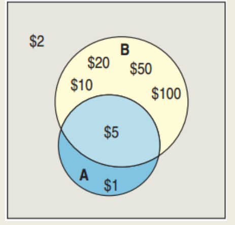
S = {$1, $2, $5, $10, $20, $50, $100}
A = {odd numbered value} = {$1, $5}
B = {bill with a building} = {$5, $10, $20, $50, $100}
Why is \(P(A \text{ or } B) \ne P(A) + P(B)\)?
Answer: A and B are not disjoint.
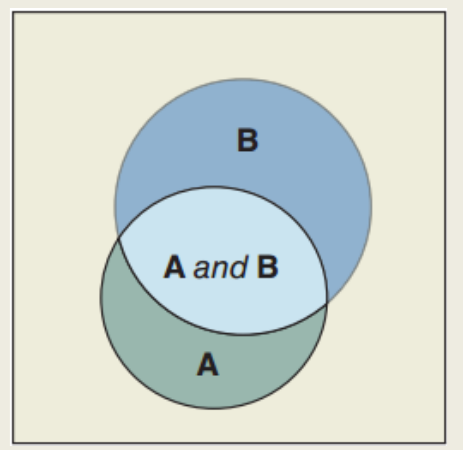
The intersection A and B = {$5} is double counted.
To find \(P(A \text{ or } B)\), subtract \(P(A \text{ and } B)\).
The General Addition Rule
\[P(A \text{ or } B) = P(A) + P(B) - P(A \text{ and } B)\]
The General Addition Rule in words: Add the probabilities of the two events and then subtract the probability of their intersection.
Now imagine that you roll the die 10 times obtaining: {5,6,4,5,3,2,1,2,4,6}
The sample mean, for this specific sample, is 3.8.
Imagine that you take another sample; this time the mean is 3.4. You keep taking samples and calculating the mean; ultimately the mean of the means will converge to 3.5.
15.2
Spread: The Standard Deviation
Review: measure of spread for data
For data, we calculated the sample variance by first computing the deviation from the mean, then squaring it and averaging it.
\[s^2 = \frac{\sum (y - \bar{y})^2}{n - 1}\]
The sample standard deviation is the square root of the sample variance
→ The standard deviation expresses the average distance from the mean
Formulas for population variance and sample variance are different.
15.3
Shifting and Combining Random Variables
More About Means and Variances
Adding or subtracting a constant from data shifts the mean but doesn’t change the variance or standard deviation:
\[E(X \pm c) = E(X) \pm c \qquad Var(X \pm c) = Var(X)\]
Example: Consider everyone in a company receiving a $5000 increase in salary.
15.4
Continuous Random Variables
Continuous Random Variables
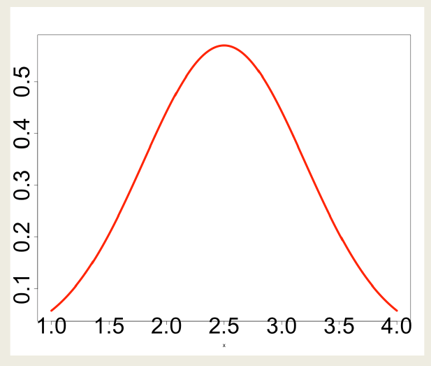
Random variables that can take on any value in a range of values are called continuous random variables.
x <-seq(1,4,length=1000)y <-dnorm(x,mean=2.5, sd=0.7)plot(x,y,type="l",lwd=6,cex.axis=4,col=("red"))
Probability as an area
Random variables that can take on any value in a range of values are called continuous random variables.
The fact that we are talking about any value has some consequences.
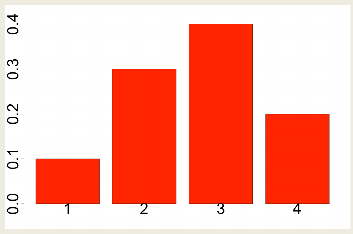
Let’s take a step back, looking at a discrete distribution again.
Which is bigger, \(P(X = 1 \text{ or } X = 2)\) or \(P(X = 3 \text{ or } X = 4)\)?
We can think about probability as an area.
Continuous Random Variables
Random variables that can take on any value in a range of values are called continuous random variables.
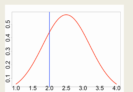
We can think about probability as an area under a curve…
Any value → any single value won’t have a probability!
But continuous random variables do have means (expected values) and variances.
What Can Go Wrong?
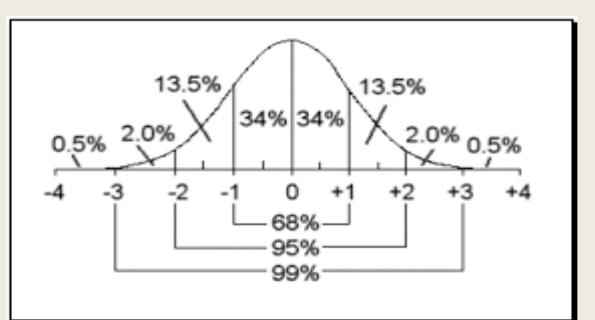
Don’t assume everything’s Normal.
You must Think about whether the Normality Assumption is justified.
What Can Go Wrong?
Probability models are still just models.
Models can be useful, but they are not reality.
Question probabilities as you would data, and think about the assumptions behind your models.
If the model is wrong, so is everything else.
Chapter 16
Probability Models
Overview
Is a result typical or unusual?
How do we build a probability model for our data?
Random variable
There are many different distributions we can define and use, discrete or continuous.
Examples:
Discrete: geometric or binomial
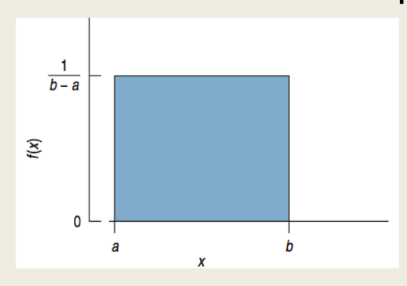
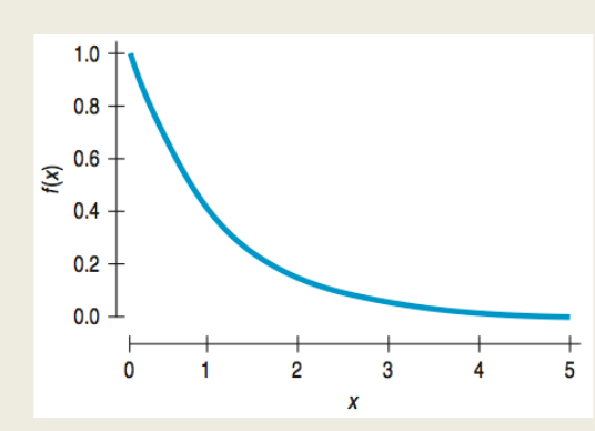
Continuous: normal, uniform, exponential
Focus on binomial and normal distributions
Before we do that, we need to define a basic “experiment”, a Bernoulli trial
16.1
Bernoulli Trials
Bernoulli Trials
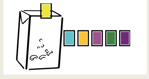
You’re collecting cards from cereal boxes. You don’t care about completing the whole card collection, but you’ve just got to have the blue card.
How many boxes do you expect you’ll have to open before you find the blue card?
We’ll keep the assumption that cards are distributed at random and we’ll trust the manufacturer’s claim that 20% of the cards are blue.
So, when you open the box, the probability that you succeed in finding blue card is 0.20. Now we’ll call the act of opening each box a trial, and note that:
Bernoulli Trials
There are only two possible outcomes (called success and failure) on each trial. Either you get the blue card (success), or you don’t (failure).
The probability of success, denoted p, is the same on every trial. Here p = 0.20.
The trials are independent. Finding the blue card in the first box does not change what might happen when you reach for the next box.
Situations like this occur often and are called Bernoulli trials.
Bernoulli Trials
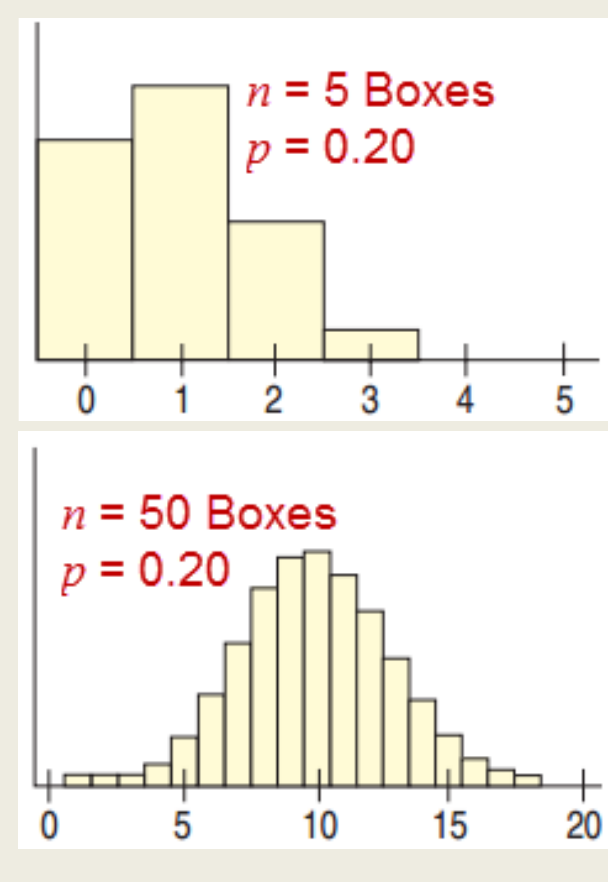
Since the blue card is in 20% of the boxes, we expect we will need to open, on average, five boxes:
\[E(Y) = \frac{1}{0.2} = 5 \text{ boxes}\]
Not easy to prove!
Common Examples of Bernoulli Trials
tossing a coin
looking for defective products rolling off an assembly line
shooting free throws in a basketball game
16.2
The Geometric Model
The Geometric Model: How long does it take?
We want to model how long it will take to achieve the first success in a series of Bernoulli trials.
The model that tells us this probability is called the Geometric probability model.
Geometric Probability Model for Bernoulli Trials: GEOM(n, p)
p = probability of success
q = 1 – p = probability of failure
X = number of trials until the first success occurs
\[P(X = x) = q^{x-1} p\]
Expected value: \(E(X) = \mu = \dfrac{1}{p}\)
Standard deviation: \(\sigma = \sqrt{\dfrac{q}{p^2}}\)
Independence – The 10% Condition
One of the important requirements for Bernoulli trials is that the trials be independent.
The 10% Condition: Bernoulli trials must be independent. If that assumption is violated, it is still okay to proceed as long as the sample is smaller than 10% of the population.
Universal Blood Donors
6% of all people are O−, Universal Donors.
If donors line up at random for a blood drive, how many do you expect to examine before you find someone who has O-negative blood?
What’s the probability that the first O-negative donor found is one of the first four people in line?
Plan: Either success (O−) or Failure (not O−); p = 0.06, independent, 10% condition
Variable: X = no. of donors until O−
Model: X is Geom(0.06)
Universal Blood Donors
Mechanics: Calculate probability that X = 1, 2, 3, 4
Conclusion: Blood drives such as this one expect to examine an average of 16.7 people to find a universal donor. About 22% of the time there will be one within the first 4 people in line.
16.3
The Binomial Model
The Binomial Model: How many successes?
A Binomial probability model describes the number of successes in a specified number of trials.
It takes two parameters to specify this model: the number of trials n and the probability of success p.
Binomial Probability Model for Bernoulli Trials: BINOM(n, p)
6% of all people are O−. If 20 donate at the blood drive, find the mean and sd of the number of universal donors and find the probability that 2 or 3 are O−.
Plan: Either success (O−) or Failure (not O−); p = 0.06, independent, 10% condition. Therefore binomial
Variable: X = no. of O−, n = 20 people
Model: X is Binom(20, 0.06)
Universal Blood Donors
6% of all people are O−. If 20 donate at the blood drive, find the mean and sd of # of universal donors and find the probability that 2 or 3 are O−.
6% of all people are O−. If 20 donate at the blood drive, find the mean and sd of # of universal donors and find the probability that 2 or 3 are O−.
Conclusion: In groups of 20 randomly selected blood donors, I expect to find an average of 1.2 universal blood donors with a standard deviation of 1.06. There is about a 31% chance that 2 or 3 of the 20 donors are O−.
16.4
Approximating the Binomial with the Normal Model
The Trouble with Large Sample Sizes
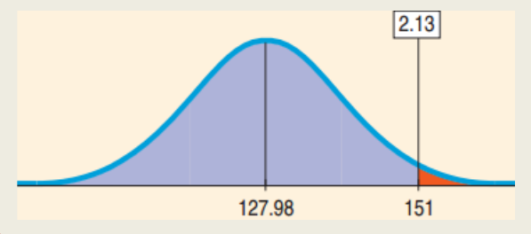
The Tennessee Red Cross has 32,000 donors and needs at least 1850 that are O−. Will they run out?
The computations involve ridiculously large numbers.
“At least” requires \(P(X = 1850)\), \(P(X = 1851)\), all the way up to \(P(X = 32{,}000)\).
Mean \(= np = 1920\)
\[SD = \sqrt{npq} \approx 42.48\]
The Solution for Large Sample Sizes
The Tennessee Red Cross has 32,000 donors and needs at least 1850 that are O−. Will they run out (less than)?