Quantitative Methods

Lecture 9

Serena DeStefani

2020-07-20

Quantitative Methods

Serena DeStefani – Lecture 9 – 7/20/2020

Announcements

Tomorrow afternoon all HW assignments returned
Review on Wednesday: please email questions/ topic for review
Midterm on Thursday
40 questions, 45 points
Four problems + theory questions

Review: Chapter 15

Random Variables

Overview

Till now we have mostly dealt with probabilities.
Now: is a result typical or unusual?
We are about to start a long journey to try to answer this question!
What we want: a probability model (or probability distribution) for our data → compare
How do we build it?
We use the concept of random variable

Random variables

A random variable, X, is a variable whose possible values are the numerical outcomes of the model of a random phenomenon.

We use a capital letter, like X, to denote a random variable.
A particular value of a random variable will be denoted with the corresponding lower case letter, in this case x.

Discrete and continuous random variables

There are two types of random variables:

A discrete random variable is one which may take on only a countable number of distinct values such as 0,1,2,3,4
- Example: Number of children in a family: 0,1,2,3,4,5,6,7…?
A continuous random variable can take any numeric value within a range of values.
- Example: Cost of books per term: Any number from $0 to $400?

Discrete probability distribution example

Suppose a discrete variable X can take the values 1, 2, 3, or 4.

The probabilities associated with each outcome are described by the following table:

data <- c(0.1,0.3,0.4,0.2)
barplot(data,
        names.arg=c("1", "2", "3", "4"),
        cex.axis = 4,
        cex.names = 4,
        col=("red"))

Example (cont.)

What’s the probability that X is equal to 2 or 3?

It is the sum of the two probabilities:

$P(X = 2 \text{ or } X = 3) = P(X = 2) + P(X = 3) = 0.3 + 0.4 = 0.7$

What’s the probability that X is greater than 1?

It is equal to $1 - P(X = 1) = 1 - 0.1 = 0.9$, by the complement rule.

Probability Model and Expected Value

A probability model for a random variable consists of:

The collection of all possible values of a random variable AND
the probabilities that the values occur.

Of particular interest is the value we expect a random variable to take on, notated μ (for population mean) or E(X) for expected value.

When we looked at a dataset, we calculated the sample mean ($\bar{X}$) as average.

Formulas for population mean and sample mean are different…

What is the Population Mean/ Expected value?

The expected value of a (discrete) random variable can be found by summing the products of each possible value by the probability that it occurs:

\[\mu = E(X) = \sum x \cdot P(x)\]

E(X) = (1*0.1)+(2*0.3)+(3*0.4)+(4*0.2)

We sum the values weighted by their probabilities (or relative frequencies)

The sample mean is an average. It varies from sample to sample.

The population mean is a sum of values weighted by their probabilities. It does not vary

Expected Value and Sample Mean

Imagine you have a fair die. Knowing all the possible outcomes and their probabilities, we can calculate E(X):

$E(X) = 1 \cdot \tfrac{1}{6} + 2 \cdot \tfrac{1}{6} + ... 6 \cdot \tfrac{1}{6} = 3.5$

This number is constant.

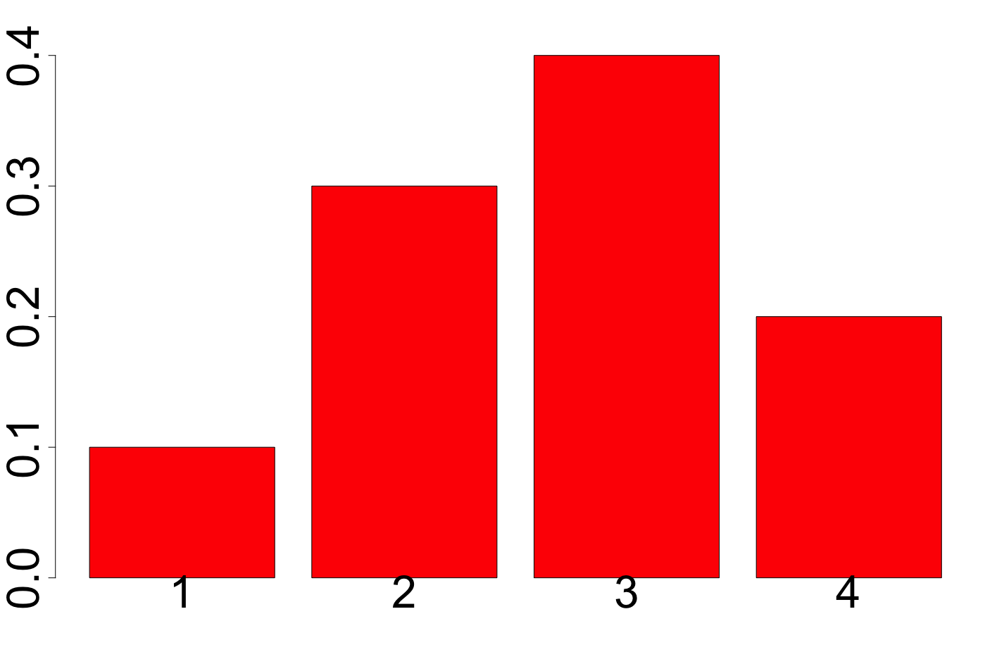
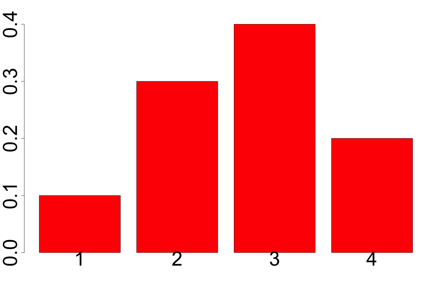
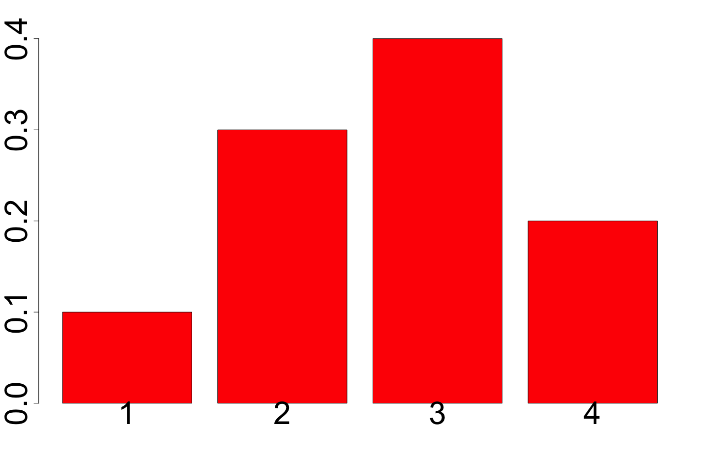
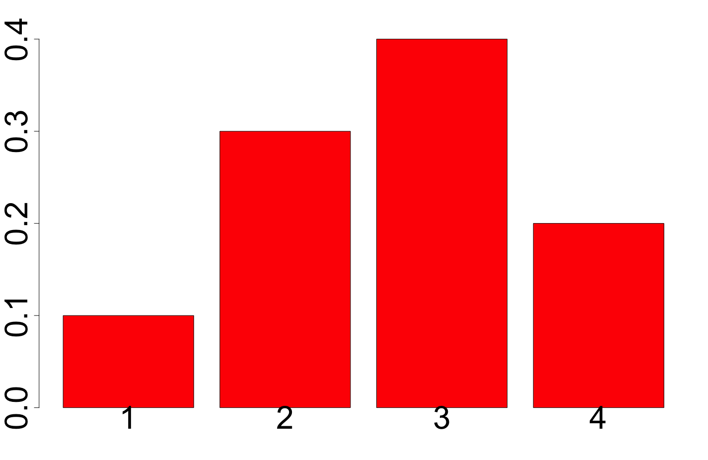
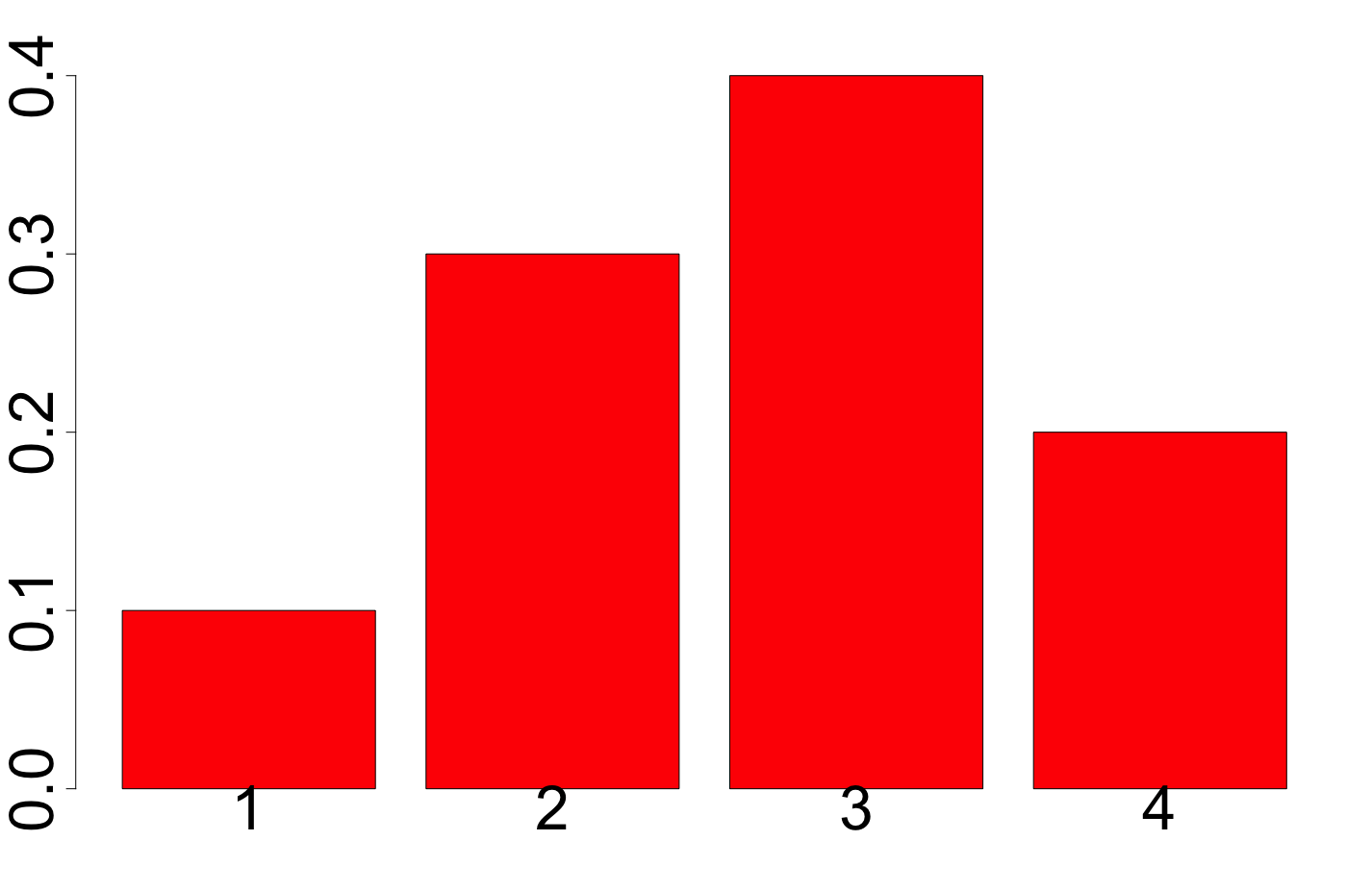
Now imagine that you roll the die 10 times obtaining:

{5,6,4,5,3,2,1,2,4,6}

The sample mean, for this specific sample, is 3.8.

Imagine that you take another sample; this time the mean is 3.4. You keep taking samples and calculating the mean; ultimately the mean of the means will converge to 3.5.

Continuous Random Variables

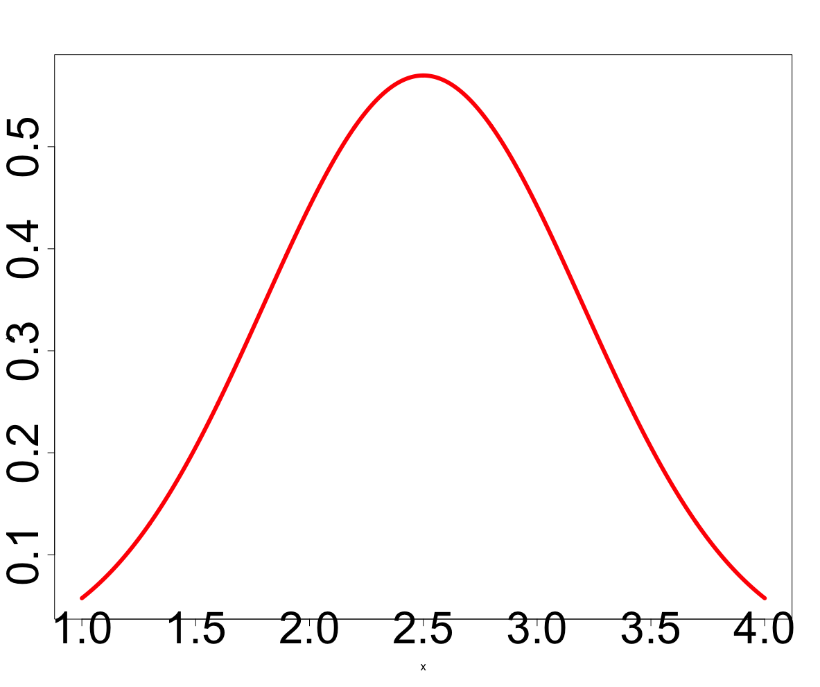
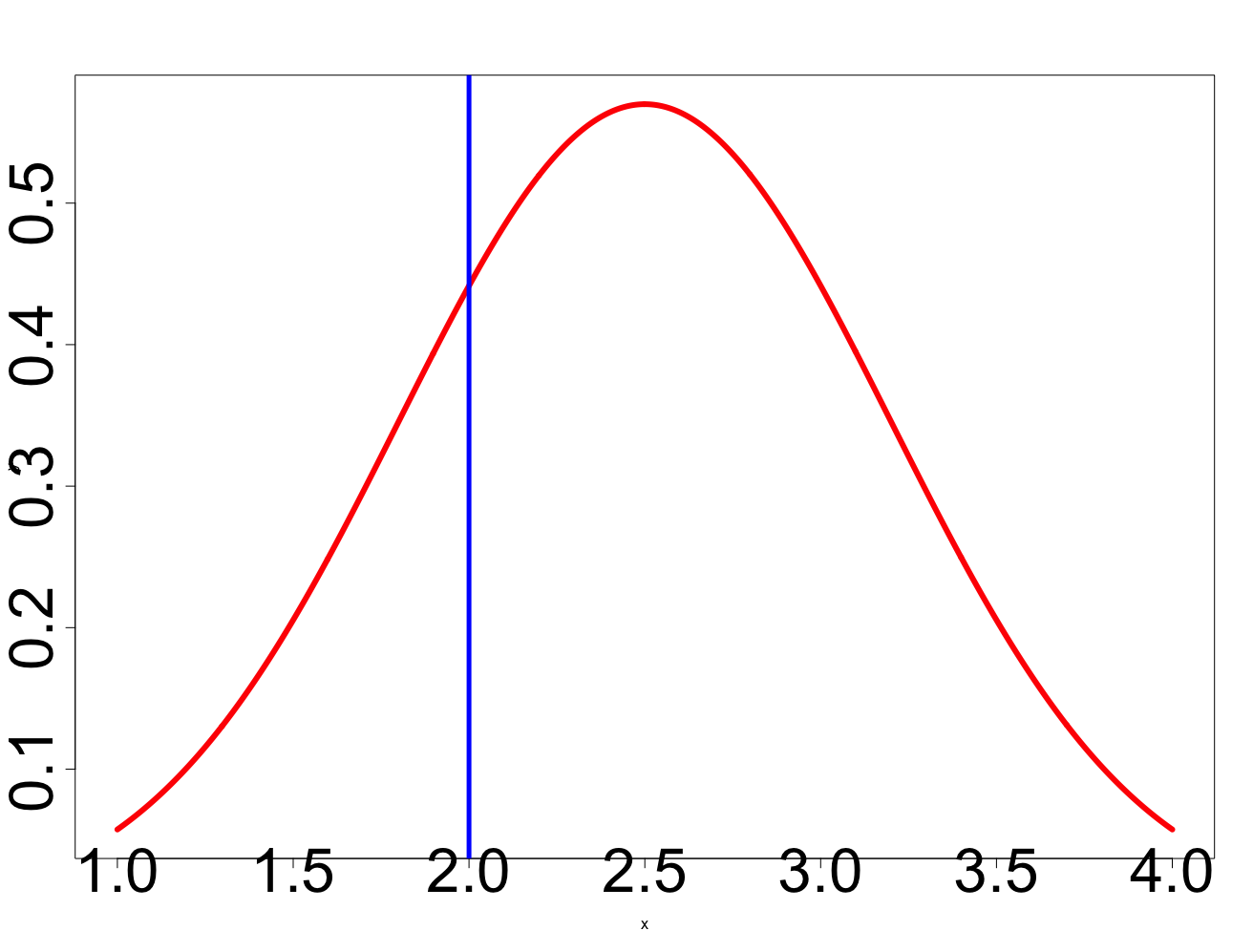
Random variables that can take on any value in a range of values are called continuous random variables.

x   <- seq(1,4,length=1000)
y   <- dnorm(x,mean=2.5, sd=0.7)
plot(x,y,
     type="l",
     lwd=6,
     cex.axis=4,
     col=("red"))

Chapter 16

Probability Models

Summary

Question: is my result likely? I need a model
How do we build a model for our data?
Random variable
→ Probability model (or probability distribution)
There are many different distributions we can define and use, discrete or continuous.
Examples:
- Discrete: geometric or binomial
- Continuous: normal, uniform, exponential
Focus on binomial and normal distributions
Before we look at distributions, we need to define a basic “experiment”, a Bernoulli trial

Continuous and Discrete Random Variables

Discrete

Continuous

Review: Bernoulli Trials

There are only two possible outcomes (called success and failure) on each trial.
The probability of success, denoted p, is the same on every trial.
The trials are independent. Obtaining a success in one trial does not influence the probability of obtaining a success in another trial.

Situations like this occur often and are called Bernoulli trials.

We saw two probability models for Bernoulli trials: the geometric model and the binomial model.

The Geometric Model

We want to model how long it will take to achieve the first success in a series of Bernoulli trials.
The model that tells us this probability is called the Geometric probability model.

Geometric Probability Model for Bernoulli Trials: GEOM(n, p)

p = probability of success

q = 1 – p = probability of failure

X = number of trials until the first success occurs

\[P(X = x) = q^{x-1}p\]

Expected value: $E(X) = \mu = \dfrac{1}{p}$

Standard deviation: $\sigma = \sqrt{\dfrac{q}{p^2}}$

The Binomial Model

A Binomial probability model describes the number of successes in a specified number of trials.
It takes two parameters to specify this model: the number of trials n and the probability of success p.
A binomial model can be used to model a survey answer, or any binary proportion

Binomial Probability Model for Bernoulli Trials: BINOM(n, p)

n = number of trials

p = probability of success

q = 1 – p = probability of failure

X = number of successes in n trials

\[P(X = x) = {}_{n}C_{x}\, p^{x} q^{n-x}, \qquad {}_{n}C_{x} = \frac{n!}{x!\,(n-x)!}\]

Mean: $\mu = np$

Standard deviation: $\sigma = \sqrt{npq}$

The Solution for Large Sample Sizes

When the sample of our binomial model is too big, calculating probabilities becomes too complicated → use a normal model to approximate it.

First we calculate mean and SD according to the binomial model.

Then we use a normal model with the same mean and standard deviation as a very good approximation.

If we have a normal model, we can use z-scores to calculate probabilities.

For the approximation to work, we need at least 10 successes and 10 failures.

Example: Spam and the Normal Approximation to the Binomial

A report found 91% of email messages are spam (probability email is real: 0.09)

Only 151 of 1422 emails got through your spam filter. Might the filter be too aggressive?

What is the probability that no more than 151 of the emails are real messages?
These emails represent less than 10% of all emails.
np = (1422)(0.09) = 127.98 $\ge$ 10
nq = (1422)(0.91) = 1294.02 $\ge$ 10
Yes, the Normal model is a good approximation.

Example: Spam and the Normal Approximation to the Binomial

What is the probability that no more than 151 of the emails are real messages?
$\mu = np = 127.98$
$\sigma = \sqrt{npq} \approx 10.79$

\[P(X \le 151) \approx P\left(z \le \frac{151 - 127.98}{10.79}\right) \approx P(z \le 2.13) \approx 0.9834\]

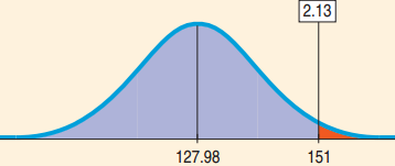
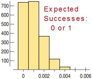
There is over a 98% chance that no more than 151 of them were real messages. The filter may be working.

Chapter 17

Sampling Distribution Models

17.1

Sampling Distribution of a Proportion

Sampling About Climate Change

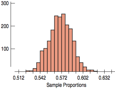
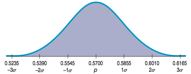
According to a Gallup poll of 1022 Americans, 57% believe that climate change is due to human activity.

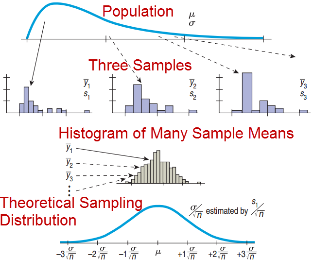
If many surveys were done of 1022 Americans, we could calculate the sample proportion for each.

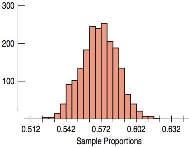
The histogram shows the distribution of a simulation of 2000 sample proportions.
The distribution of all possible sample proportions from samples with the same sample size is called the sampling distribution.

Sampling Distributions

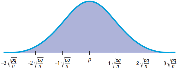
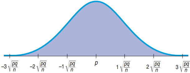
Sampling Distribution for Proportions

Symmetric
Unimodal
Centered at p
The sampling distribution follows the Normal model.

What does the sampling distribution tell us?

The sampling distribution allows us to make statements about where we think the corresponding population parameter is and how precise these statements are likely to be.

Sampling Distribution for Smoking

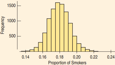
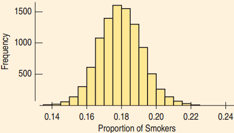
18% of US adults smoke. How much would we expect the proportion of smokers in a sample of size 1000 to vary from sample to sample?

We run a simulation
# from 1 to 100
# from 1 to 18: smokers
draw 10,000 samples of 1000
Histogram: simulation’s results

Sampling Distribution for Smoking

18% of US adults smoke. How much would we expect the proportion of smokers in a sample of size 1000 to vary from sample to sample?

We run a simulation
Histogram: simulation’s results
The mean is 0.18 = the population proportion.
The standard deviation was calculated as 0.0122.

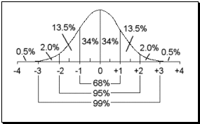
Roughly Normal: 68-95-99.7 rule works.
95% of all proportions are within 0.0244 of the mean.
This is very close to the value found: 95.41%

From One Sample to Many Samples

Distribution of One Sample

Variable was the answer to the survey question or the result of an experiment.
Proportion is a fixed value that comes from the one sample.

Sampling Distribution

Variable is the proportion that comes from the entire sample.
Many proportions that differ from one to another, each coming from a different sample.

Mean and Standard Deviation

Sampling Distribution for Proportions

$\text{Mean} = p$
$\sigma(\hat{p}) = \dfrac{\sqrt{npq}}{n} = \sqrt{\dfrac{pq}{n}}$
$N\left(p, \sqrt{\dfrac{pq}{n}}\right)$

This p is a parameter!

Instead $\hat{p}$ is a statistic!

The Normal Model for Climate Change

Population: p = 0.57, n = 1022. Sampling Distribution:

Mean = 0.57
Standard deviation $= SD(\hat{p}) = \sqrt{\dfrac{(0.57)(0.43)}{1022}} \approx 0.0155$

Smokers Revisited: Standard Error

p = 0.18, n = 1000

Standard deviation $= SD(\hat{p}) = \sqrt{\dfrac{(0.18)(0.82)}{1000}} \approx 0.0121$
Standard deviation from simulation: 0.0122

The sample-to-sample standard deviation is called the standard error or sampling variability.

The standard error is not a “real” error, since no error has been made.

17.2

When Does the Normal Model Work? Assumptions and Conditions

When Does the Normal Model Work?

Success Failure Condition: $np \ge 10$, $nq \ge 10$. There must be at least 10 expected successes and failures.
Independent trials: Check for the Randomization Condition.
10% Condition: Sample size less than 10% of the population size

Understanding Health Risks

22% of US women have a BMI that is 30 or more – a value associated with increased health risk.

Only 31 of the 200 randomly chosen women from a large college had a BMI above 30. Is this proportion unusually small?
- Randomization Condition: Yes, the women were randomly chosen.
- 10% Condition: For a large college, this is ok.
- Success Failure Condition: $31 \ge 10$, $169 \ge 10$
Yes, the Normal model can be used.

Understanding Health Risks: n = 200, p = 0.22, x = 31

\[\hat{p} = \frac{31}{200} = 0.155, \quad p = 0.22, \quad SD(\hat{p}) = \sqrt{\frac{(0.22)(0.78)}{200}} \approx 0.029\]

\[z = \frac{0.155 - 0.22}{0.029} \approx -2.24\]

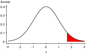
68-95-99.7 Rule: Values 2 SD below the mean occur less than 2.5% of the time. Perhaps this college has a higher proportion of healthy women, or women who lie about their weight.

Enough Lefty Seats?

13% of all people are left handed.

A 200-seat auditorium has 15 lefty seats.
What is the probability that there will not be enough lefty seats for a class of 90 students?

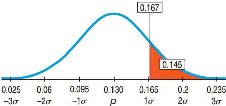
Plan: 15/90 ≈ 0.167, Want $P(\hat{p} > 0.167)$
Model:
- Independence Assumption: With respect to lefties, the students are independent.
- 10% Condition: This is out of all people.
- Success/Failure Condition: $11.7 \ge 10$, $78.3 \ge 10$

Enough Lefty Seats?

Model: $p = 0.13, \quad SD(\hat{p}) = \sqrt{\dfrac{(0.13)(0.87)}{90}} \approx 0.035$

The model is: N(0.13, 0.035)

Plot
Mechanics: $z = \dfrac{0.167 - 0.13}{0.035} \approx 1.06$

\[P(\hat{p} > 0.167) = P(z > 1.06) \approx 0.1446\]

Enough Lefty Seats?

Conclusion: There is about a 14.5% chance that there will not be enough seats for the left handed students in the class.

17.3

The Sampling Distribution of Other Statistics

The Sampling Distribution for Others

There is a sampling distribution for any statistic, but the Normal model may not fit.
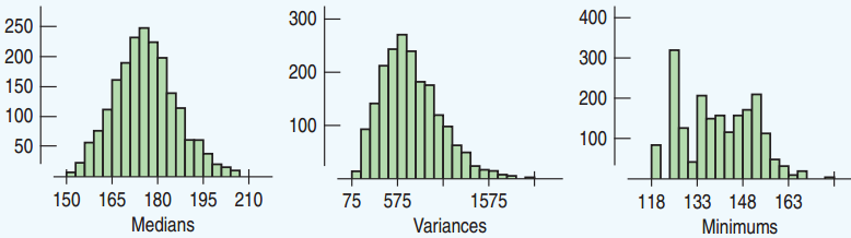
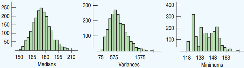
Below are histograms showing results of simulations of sampling distributions.

The Sampling Distribution For Others

The medians seem to be approximately Normal.
The variances seem somewhat skewed right.
The minimums are all over the place.
In this course, we will focus on the proportions and the means.

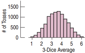
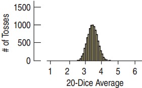
Sampling Distribution of the Means

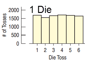
For 1 die, the distribution is Uniform.
For 3 dice, the sampling distribution for the means is closer to Normal.
For 20 dice, the sampling distribution for the means is very close to normal. The standard deviation is much smaller.

17.4

The larger the sample, the better the approximation will be.

The Central Limit Theorem

The Central Limit Theorem

The sampling distribution of any mean becomes nearly Normal as the sample size grows.

Requirements

Independent
Randomly collected sample

The sampling distribution of the means is close to Normal if either:

Large sample size
Population close to Normal

How Normal?

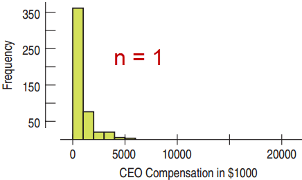
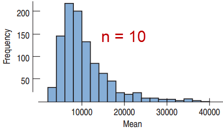
Population Distribution and Sampling Distribution of the Means

Population Distribution

Normal
Uniform
Bimodal
Skewed

Sampling Distribution for the Means

→ Normal (any sample size)
→ Normal (large sample size)
→ Normal (larger sample size)
→ Normal (larger sample size)

Binomial Distributions and the Central Limit Theorem

Consider a Bernoulli trial as quantitative:
- Success = 1
- Failure = 0
- The mean of many trials is just $\hat{p}$.
This distribution of a single trial is far from Normal.
By the Central Limit Theorem, the Binomial distribution is approximately normal for large sample sizes.

Standard Deviation of the Means

Which would be more unusual: a student who is 6’9” tall in the class or a class that has mean height of 6’9”?
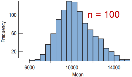
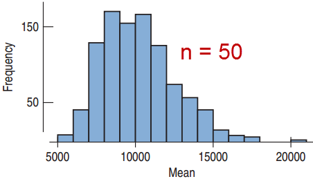
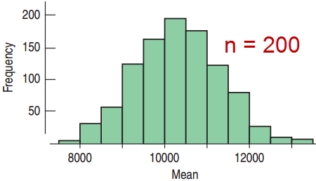
The sample means have a smaller standard deviation than the individuals.
The standard deviation of the sample means goes down by the square root of the sample size:

\[SD(\bar{y}) = \frac{\sigma}{\sqrt{n}}\]

The Sampling Distribution Model for a Mean

When a random sample is drawn from a population with mean $\mu$ and standard deviation $\sigma$, the sampling distribution has:

Mean: $\mu$
Standard Deviation: $\dfrac{\sigma}{\sqrt{n}}$
For large sample size, the distribution is approximately normal regardless of the population the random sample comes from.
The larger the sample size, the closer to Normal.

Low BMI Revisited

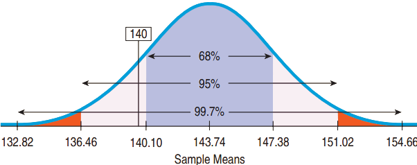
The 200 college women with the low BMI reported a mean weight of only 140 pounds. For all 18-year-old women, $\mu$ = 143.74 and $\sigma$ = 51.54. Does the mean weight seem exceptionally low?

Randomization Condition: The women were a random sample with weights independent.
Sample size Condition: Weights are approximately Normal. 200 is large enough.

Low BMI Revisited

Mean and Standard Deviation of the sampling distribution

\[\mu(\bar{y}) = 143.7 \qquad SD(\bar{y}) = \frac{\sigma}{\sqrt{n}} = \frac{51.54}{\sqrt{200}} \approx 3.64\]

The 68-95-99.7 rule suggests that the mean is low but not that unusual. Such variability is not extraordinary for samples of this size.

Too Heavy for the Elevator?

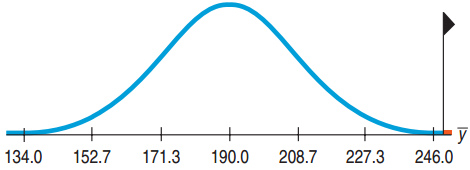
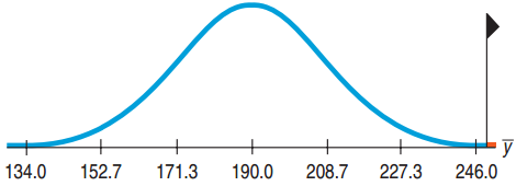
Mean weight of US men is 190 lb, the standard deviation is 59 lb. An elevator has a weight limit of 10 persons or 2500 lb. Find the probability that 10 men in the elevator will overload the weight limit.

Plan: 10 over 2500 lb same as their mean over 250.
Model:
- Independence Assumption: Not random, but probably independent.
- Sample Size Condition: Weight approx. Normal.

Too Heavy for the Elevator

Model: $\mu$ = 190, $\sigma$ = 59. By the CLT, the sampling distribution of $\bar{y}$ is approximately Normal:

\[\mu(\bar{y}) = 190, \; SD(\bar{y}) = \frac{\sigma}{\sqrt{n}} = \frac{59}{\sqrt{10}} \approx 18.66\]

Plot:

Too Heavy for the Elevator?

Mechanics:

\[z = \frac{\bar{y} - \mu}{SD(\bar{y})} = \frac{250 - 190}{18.66} \approx 3.215\]

\[P(\bar{y} > 250) \approx P(z > 3.21) \approx 0.0007\]

Conclusion: There is only a 0.0007 chance that the 10 men will exceed the elevator’s weight limit.

17.5

Sampling Distributions: A Summary

Sample Size and Standard Deviation

\[SD(\bar{y}) = \frac{\sigma}{\sqrt{n}} \qquad SD(\hat{p}) = \frac{\sqrt{pq}}{\sqrt{n}}\]

Larger sample size → Smaller standard deviation
Multiply n by 4 → Divide the standard deviation by 2.
Need a sample size of 100 to reduce the standard deviation by a factor of 10.

Billion Dollar Misunderstanding

Bill and Melinda Gates Foundation found that 12% of the top 50 performing schools were from the smallest 3%. They funded a transformation to small schools.

Small schools have a smaller n, thus a higher standard deviation.
Likely to see both higher and lower means.
18% of the bottom 50 were also from the smallest 3%.

Distribution of the Sample vs. the Sampling Distribution

Don’t confuse the distribution of the sample and the sampling distribution.

If the population’s distribution is not Normal, then the sample’s distribution will not be normal even if the sample size is very large.
For large sample sizes, the sampling distribution, which is the distribution of all possible sample means from samples of that size, will be approximately Normal.

Two Truths About Sampling Distributions

Sampling distributions arise because samples vary. Each random sample will contain different cases and, so, a different value of the statistic.
Although we can always simulate a sampling distribution, the Central Limit Theorem saves us the trouble for proportions and means. This is especially important when we do not know the population’s distribution.

What Can Go Wrong?

Don’t confuse the sampling distribution with the distribution of the sample.
- A histogram of the data shows the sample’s distribution. The sampling distribution is more theoretical.
Beware of observations that are not independent.
- The CLT fails for dependent samples. A good survey design can ensure independence.
Watch out for small samples from skewed or bimodal populations.
- The CLT requires large samples or a Normal population or both.

Chapter 18

Confidence Intervals for Proportions

18.1

A Confidence Interval

Mean and Standard Deviation

Sampling Distribution for Proportions

$\text{Mean} = p$
$\sigma(\hat{p}) = \dfrac{\sqrt{npq}}{n} = \sqrt{\dfrac{pq}{n}}$
$N\left(p, \sqrt{\dfrac{pq}{n}}\right)$

Standard Deviation for a Proportion?

What is the sampling distribution?

Usually we do not know the population proportion p.
We cannot find the standard deviation of the sampling distribution: $\sqrt{\dfrac{pq}{n}}$
After taking a sample, we only know the sample proportion, which we use as an approximation.
The sample-to-sample standard deviation is called the standard error or sampling variability
The standard error is given by $SE(\hat{p}) = \sqrt{\dfrac{\hat{p}\hat{q}}{n}}$

Facebook Daily Status Updates

A recent survey found that 48 of 156 or 30.8% update their Facebook status daily.

\[SE(\hat{p}) = \sqrt{\frac{\hat{p}\hat{q}}{n}} = \sqrt{\frac{(0.308)(0.692)}{156}} \approx 0.037\]

The sampling distribution is approximately normal.

Facebook: true population proportion?

A recent survey found that 48 of 156 or 30.8% update their Facebook status daily.

This is the sample proportion
What is the true population proportion?
To find it, we need to make an inference using the sampling distribution we just found, based on SE

Interpreting this Normal Curve

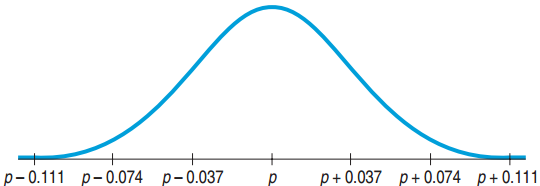
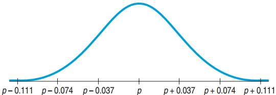
By normality, about 95% of all possible samples of 156 young Facebook users will have $\hat{p}$’s within 2 SE (0.037) of p
If $\hat{p}$ is close to p, then p is close to $\hat{p}$.

If you stand at $\hat{p}$, then you can be 95% sure that p is within 2 SE’s from where you are standing.
→ Our confidence interval: (0.234, 0.382)

What You Can Say About p if You Know $\hat{p}$

We don’t know exactly what percent of all Facebook users update their status daily, but the interval from 23.4% and 38.2% probably contains the true proportion.

Note, we admit we are unsure about both the exact proportion and whether it is in the interval.

We are 95% confident that between 23.4% and 38.2% of all Facebook users update their status daily.

Notice “% confident” and an interval rather than an exact value are stated.

What You Cannot Say About p if You Know $\hat{p}$

30.8% of all Facebook users update their status daily.

We can’t make such absolute statements about p.

It is probably true that 30.8% of all Facebook users update their status daily.

We still cannot commit to a specific value for p, only a range.

We don’t know exactly what percent of all Facebook users update their status daily, but we know it is within the interval 30.8% ± 2 x 3.7%.

We cannot be certain it is in this interval.

Naming the Confidence Interval

This confidence interval is a one-proportion z-interval.

“One” since there is a single survey question.
“Proportion” since we are interested in the proportion of Facebook users who update their status daily.
“z-interval” since the distribution is approximately normal.

18.2

Interpreting Confidence Intervals: What Does 95% Confidence Really Mean?

Capturing a Proportion

The confidence interval may or may not contain the true population proportion.
Consider repeating the study over and over again, each time with the same sample size.
- Each time we would get a different $\hat{p}$.
- From each $\hat{p}$, a different confidence interval could be computed.
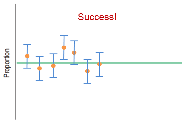
- About 95% of these confidence intervals will capture the true proportion.
- 5% will not.

Simulating Confidence Intervals

Confidence Intervals

There are a huge number of confidence intervals that could be drawn.

In theory, all the confidence intervals could be listed.
95% will “work” (capture the true proportion).
5% will not capture the true proportion.

What about our confidence interval (0.234, 0.382)?

We will never know whether it captures the population proportion.

“Statistics Means Never Having to Say You Are Certain”

Facebook Status Updates

Technically Correct

I am 95% confident that the interval from 23.4% to 38.2% captures the true proportion of Facebook users who update daily.

More Casual But Fine

I am 95% confident that between 23.4% and 38.2% of Facebook users update daily.

18.3

Margin of Error: Certainty vs. Precision

Margin of Error

Confidence interval for a population proportion:

\[\hat{p} \pm 2SE(\hat{p})\]

The distance, $2SE(\hat{p})$, from $\hat{p}$ is called the margin of error.
Confidence intervals also work for means, regression slopes, and others. In general, the confidence interval has the form

\[\text{Estimate} \pm ME\]

Certainty vs. Precision

Instead of a 95% confidence interval, any percent can be used.
Increasing the confidence (e.g. 99%) increases the margin of error.
Decreasing the confidence (e.g. 90%) decreases the margin of error.

Confidence Interval on Global Warming

Yale and George Mason University interviewed 1010 US adults about beliefs and attitudes on global warming. They presented a 95% confidence interval on the proportion who think there is disagreement among scientists.

Had the polling been done repeatedly, 95% of all random samples would yield confidence intervals that contain the true population proportion of all US adults who believe there is disagreement among scientists.

Yale/George Mason Study Revisited

The poll of 1010 adults reported a margin of error of 3%.

(by convention, 95% with “worst case” ME based on p = 0.5)

How was the 3% computed?

\[SE(\hat{p}) = \sqrt{\frac{(0.5)(0.5)}{1010}} \approx 0.0157\]

For 95% confidence

\[ME = 2(0.0157) = 0.031\]

The margin of error is close to 3%.

Critical Values

For a 95% confidence interval, the margin of error was 2SE.
- The 2 comes from the normal curve.
- 95% of the area is within about 2SE from the mean.
In general the number of SE is called the critical value. Since we use the normal distribution here we denote it z*
To be more precise, z* for 95% CI is 1.96

Finding the Critical Value

Find the critical value corresponding to 90% confidence.

90% inside gives 10% outside.
2 tails outside with 10% means 1 tail with 5% or 0.05.
The critical value is about z* = 1.645.

Finding the Margin of Error (Take 2)

Yale/George Mason Poll: 1010 US adults, 40% think scientists disagree about global warming. At 95% confidence ME = 3%.

Find the margin of error at 90% confidence.

\[SE(\hat{p}) = \sqrt{\frac{(0.4)(0.6)}{1010}} \approx 0.0154\]

For 90%, z* ≈ 1.645: ME = (1.645)(0.0154) = 0.025.
This gives a smaller margin of error which is good.
Drawback: lower level of confidence which is bad

18.4

Assumptions and Conditions

Independence and Sample Size

Independence Condition
- If data is collected using SRS or a randomized experiment → Randomization Condition
- Some data values do not influence others.
- Check for the 10% Condition: The sample size is less than 10% of the population size.
Success/Failure Condition
- There must be at least 10 successes.
- There must be at least 10 failures.

One-Proportion z-Interval

First check for randomization, independence, 10%, and conditions on sample size.
Confidence level C, sample size n, proportion $\hat{p}$.
Confidence interval: $\hat{p} \pm z^{*}SE(\hat{p})$

\[SE(\hat{p}) = \sqrt{\frac{(\hat{p})(\hat{q})}{n}}\]

z*: the critical value that specifies the number of SE’s needed for C% of random samples to yield confidence intervals that capture the population proportion.

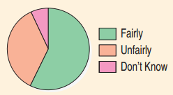
Do You Believe the Death Penalty is Applied Fairly?

Sample size: 510
Answers:
- 58% “Fairly”
- 36% “Unfairly”
- 7% “Don’t Know”
Construct a confidence interval for the population proportion that would reply “Fairly.”

Do You Believe the Death Penalty is Applied Fairly?

Plan: Find a 95% confidence interval for the population proportion.
Model:
- Randomization: Randomly selected by Gallup Poll
- 10% Condition: Population is all Americans
- Success/Failure Condition
  - (510)(0.58) = 296 > 10, (510)(0.42) = 214 > 10
- Use the Normal Model to find a one-proportion z-interval.

Do You Believe the Death Penalty is Applied Fairly?

Mechanics: n = 510, $\hat{p} = 0.58$

\[SE(\hat{p}) = \sqrt{\frac{(0.58)(0.42)}{510}} \approx 0.022\]

z* ≈ 1.96
ME ≈ (1.96)(0.022) ≈ 0.043
The 95% Confidence Interval is: 0.58 ± 0.043 or (0.537, 0.623)

Do You Believe the Death Penalty is Applied Fairly?

Conclusion: I am 95% confident that between 53.7% and 62.3% of all US adults think that the death penalty is applied fairly.

What Sample Size?

\[ME = z^{*}\sqrt{\frac{\hat{p}\hat{q}}{n}}\]

For example, to ensure a ME < 3%:
For 95%, z* = 1.96
Values that make ME largest are $\hat{p} = 0.5, \; \hat{q} = 0.5$

\[0.03 = 1.96\sqrt{\frac{(0.5)(0.5)}{n}}\]

Solving for n, gives n ≈ 1067.1.
We need to survey at least 1068 to ensure a ME less than 0.03 for the 95% confidence interval.

The Yale/George Mason Survey and Sample Size

Poll: 40% believe scientists disagree on global warming.

For a follow-up survey, what sample size is needed to obtain a 95% confidence interval with ME $\le$ 2%?

\[ME = z^{*}\sqrt{\frac{\hat{p}\hat{q}}{n}} \qquad 0.02 = 1.96\sqrt{\frac{(0.4)(0.6)}{n}}\]

n ≈ 2304.96
The group will need at least 2305 respondents.

Thoughts on Sample Size and ME

Obtaining a large sample size can be expensive and/or take a long time.
For a pilot study, ME = 10% can be acceptable.
For full studies, ME $\le$ 5% is better.
Public opinion polls typically use ME = 3%, n = 1000.
If p is expected to be very small such as 0.005, then much smaller ME such as 0.1% is required.

Credit Cards and Sample Size

A pilot study showed that 0.5% of credit card offers in the mail end up with the person signing up.

To be within 0.1% of the true rate with 95% confidence, how big does the test mailing have to be?

\[ME = z^{*}\sqrt{\frac{\hat{p}\hat{q}}{n}} \qquad 0.001 = 1.96\sqrt{\frac{(0.005)(0.995)}{n}}\]

n ≈ 19,111.96
The test mailing should include at least 19,112 offers.

What Can Go Wrong?

Don’t claim other samples will agree with yours.

Wrong: In 95% of samples, between 43% and 51% agree with decriminalization of marijuana.

Don’t be certain about the parameter.

Wrong: Between 23% and 38% of Facebook users update daily. Don’t forget to include the confidence.

Don’t forget that it’s about the parameter (not the statistics)

Wrong: I’m 95% confident that $\hat{p}$ is between 23% and 38%. You know for sure exactly what $\hat{p}$ is.

What Can Go Wrong?

Don’t claim to know too much.

Wrong: I’m 95% confident that between 23% and 38% of all Facebook users in the world update daily. The survey was just about US residents between 18 and 22.

Do take responsibility.

Accept that you are only 95% confident, not sure.

Don’t suggest that the parameter varies.

Wrong: There is a 95% chance that the true parameter is between 23% and 38%.

What Can Go Wrong?

Do treat the whole interval equally.

The middle of the interval is not necessarily more plausible than the edges.

Beware of margins of error that are too large to be useful.

Between 10% and 90% update daily is not useful. Use a larger sample size to shrink the ME.

Watch out for biased sampling.

Biased samples produce unreliable CIs.

Think about independence

Be careful in your sample design to ensure randomization.