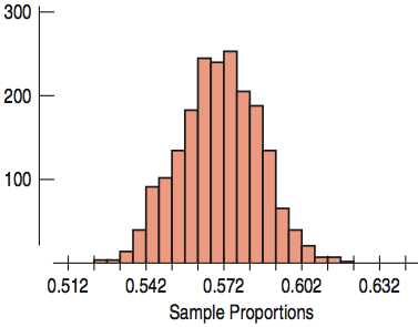
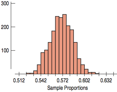
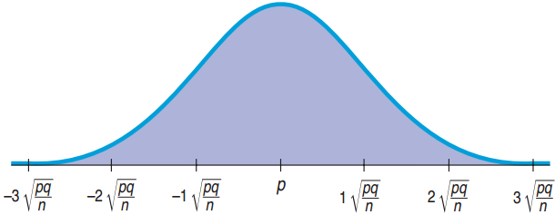
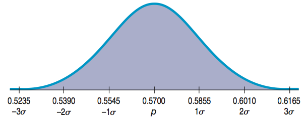
Standard deviation \(= SD(\hat{p}) = \sqrt{\dfrac{(0.57)(0.43)}{1022}} \approx 0.0155\)
The Sampling Distribution For Others
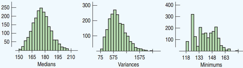
The medians seem to be approximately Normal.
The variances seem somewhat skewed right.
The minimums are all over the place.
In this course, we will focus on the proportions and the means.
The Central Limit Theorem (CLT): sampling distribution for the mean
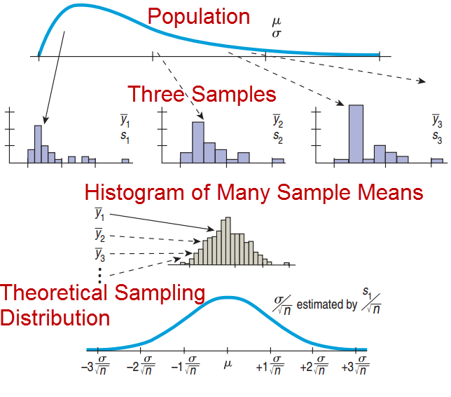
The mean of a random sample is a random variable whose sampling distribution can be approximated by a Normal model. The larger the sample, the better the approximation will be.
Population Distribution and Sampling Distribution of the Means
Population Distribution
Normal
Uniform
Bimodal
Skewed
Sampling Distribution for the Means
→ Normal (any sample size)
→ Normal (large sample size)
→ Normal (larger sample size)
→ Normal (larger sample size)
The Sampling Distribution Model for a Mean
When a random sample is drawn from a population with mean \(\mu\) and standard deviation \(\sigma\), the sampling distribution has:
Mean: \(\mu\)
Standard Deviation: \(\dfrac{\sigma}{\sqrt{n}}\)
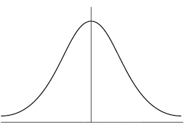
For large sample size, the distribution is approximately normal regardless of the population the random sample comes from.
The larger the sample size, the closer to Normal.
The CLT and equality
Average US salaries
How many hours you worked in a week
Average artistic level of performers
The CLT and equality
The CLT and equality
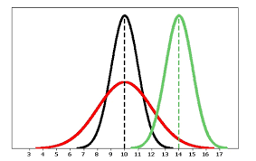
We cannot change the curve, but we can change the shape and position of the curve.
We can change our society.
This is only true for sample means. Statistics cannot tell us anything about an individual.
History of Statistics
Part 2: Galton, Pearson and Eugenics
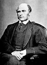
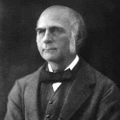
History of Statistics: Galton
Sir Francis Galton (1822 – 1911)
Darwin’s half cousin
Studied variability and hereditary traits
Problem: how to compare different features? → by their variation
Idea: features that vary together are “co-related”
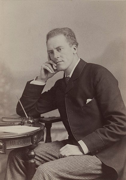
History of Statistics: Pearson
Karl Pearson (1857 – 1936)
Galton’s student
Studied correlation in the context of variability and hereditary traits
Came up with the correlation coefficient
Eugenics: Outline
Eugenics: genetic selection of human population
Eugenics in Britain
Eugenics in the United States
Nazi Germany
After WWII
Today?
What is eugenics?
Genetic selection of human population by positive or negative means
Positive: selective breeding
Negative: segregation, sterilization, killing
Evidence of Eugenics in History
Sparta: phenotypic selection through infanticide
Weak or undesirable babies were abandoned
Rome:
Fourth Table of Roman stated that deformed children would be put to death
Historical Developments
Christianity
Statistics
Evolutionary theory
Galton: a second look
Coined the word eugenics
eu “well” + genes “born”
“science of improving stock”
“I object to pretensions of natural equality.”
Galton: a second look
Inspired by Darwin’s Origin of Species
He believed societies in favor of spending resources on the weak were in opposition to natural selection
Defined eugenics as: “the science which deals with all influences that improve the inborn qualities of a race; also with those that develop them to the utmost advantage.”
His approach to eugenics was based upon social statistics
Initially eugenics was seen as a positive movement
Galton was very disappointed when he discovered the regression to the mean: very tall parents generate shorter children
Pearson: a second look
Pearson was also a proponent of eugenics.
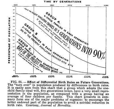
Main concern of the first eugenists: the perceived intelligence factors considered to be correlated with the social class.
“The problem of alien immigration into Great Britain, illustrated by an examination of Russian and Polish Jewish children”
“…the majority of children examined by Pearson and Moul were recent immigrants, with many actually born abroad. In Pearson’s work these children were compared to non-immigrant Gentile children, often without comment as to differing social and economic class status.”
Discounting evidence
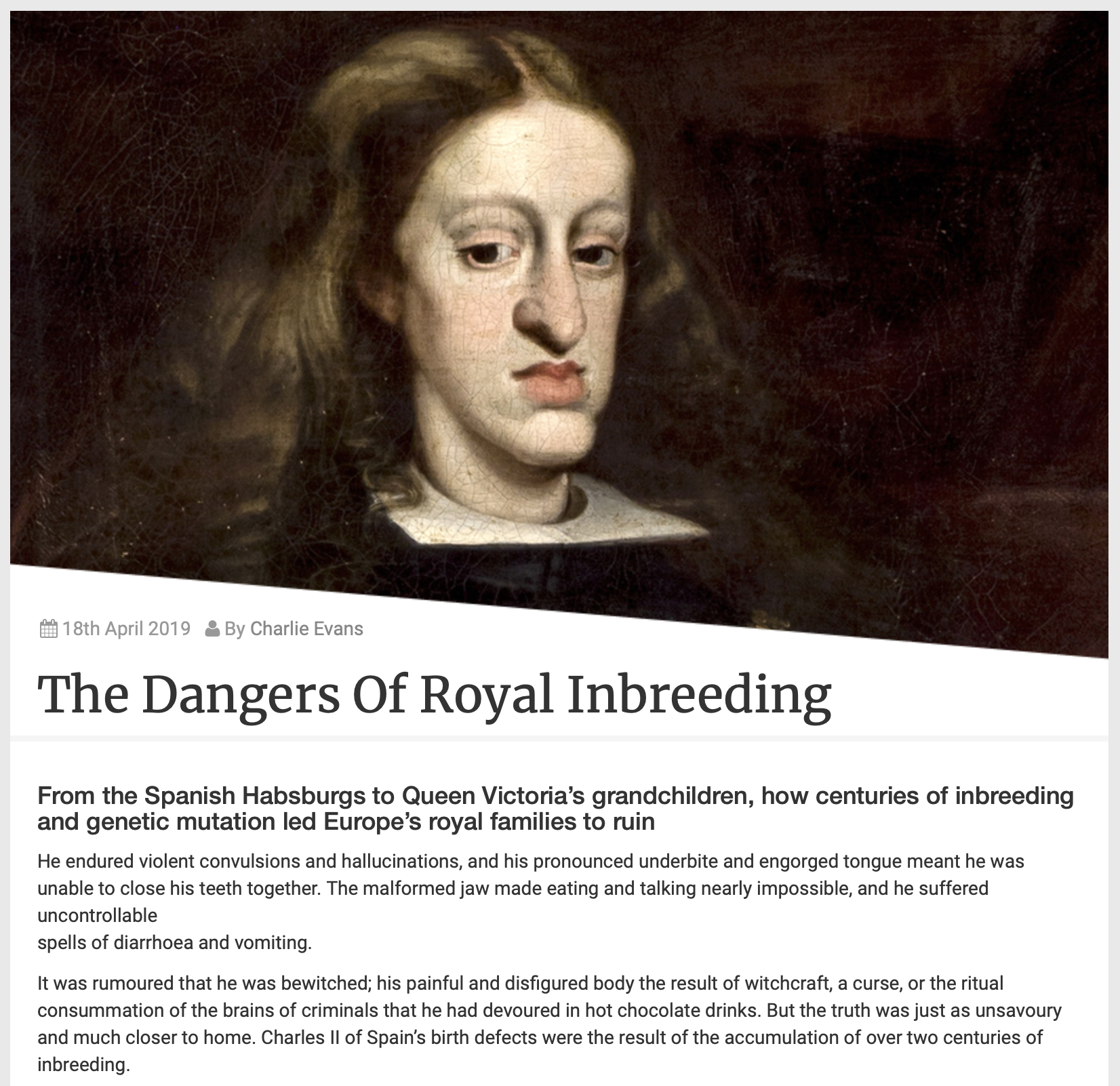
Inbreeding had brought suffering and havoc in the royal dynasties
Population problems and differences exposed by rise of mass education, and growing scale of asylums, prisons, workhouses
Emergence of new tools such as the social survey and the psychological test to rank individuals
The demographic transition
Decline in fertility
From late 19th century a fall in fertility in western nations
Concern in Britain about decline being most marked in middle-classes and among professionals
In France, fear of overall population decline by early 20th century (encourages positive forms of eugenics)
Objections to birth control and to women’s groups, birth control advocates, and even sexual liberals
The demographic transition
Other voices
Alfred Russel Wallace (1823-1913)
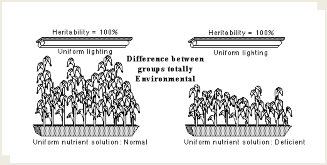
“Leave heredity alone until we have made the environment of every child from conception to death the best possible for its full and free development, and then we can begin to think about the influences of heredity, which may be small.”
U.S.: Nation building era
Heightened concern about international competition and ‘national efficiency’
Era of nation building and interest in defining the nation (e.g. post WWI)
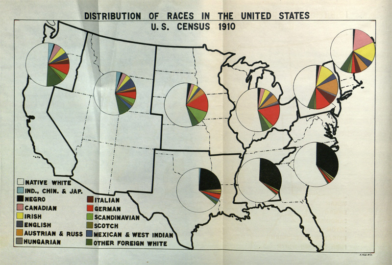
Immigrant nations concerned about racial mix
United States
Alexander Graham Bell recommended deaf individuals not be allowed to marry
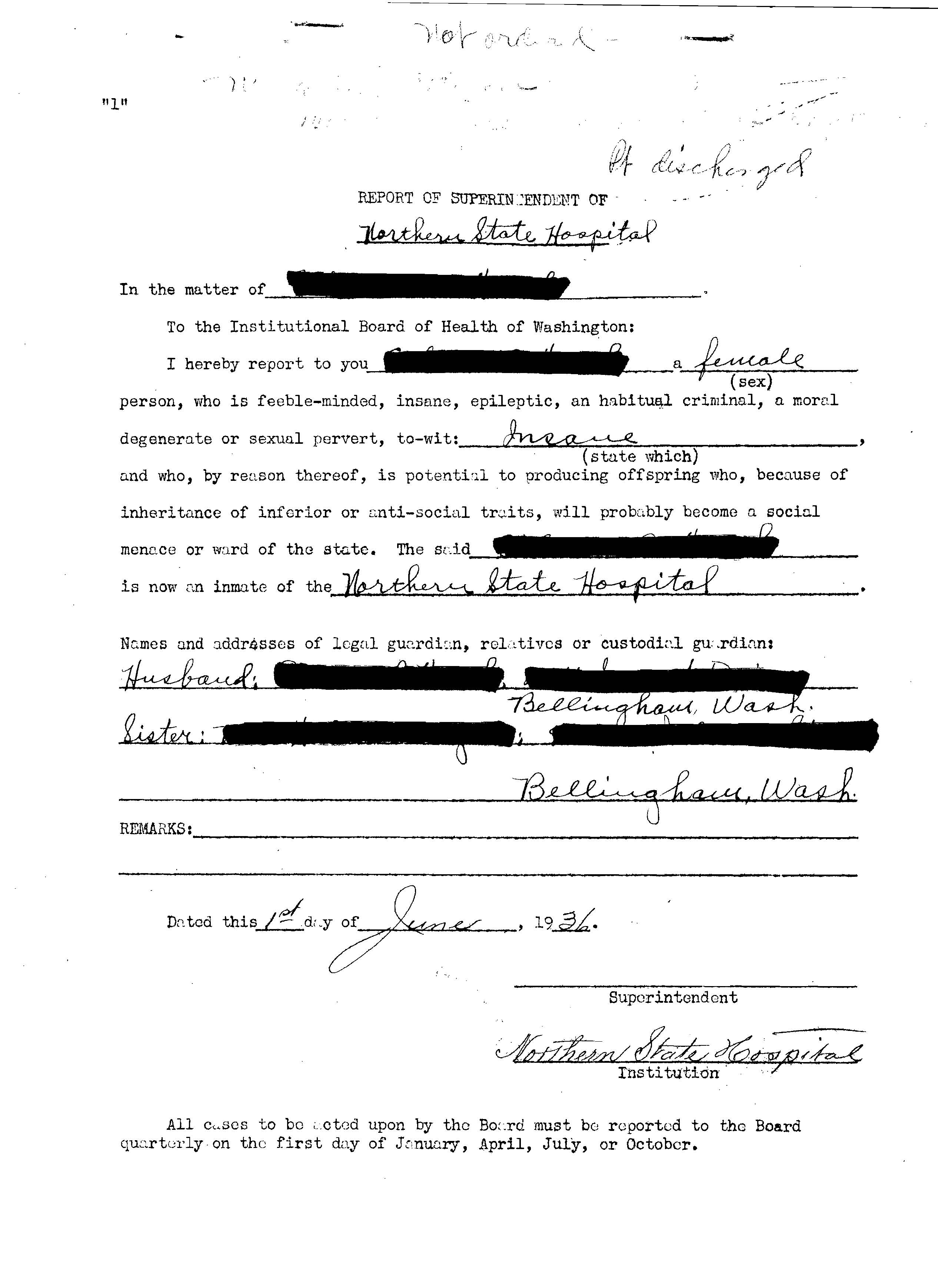
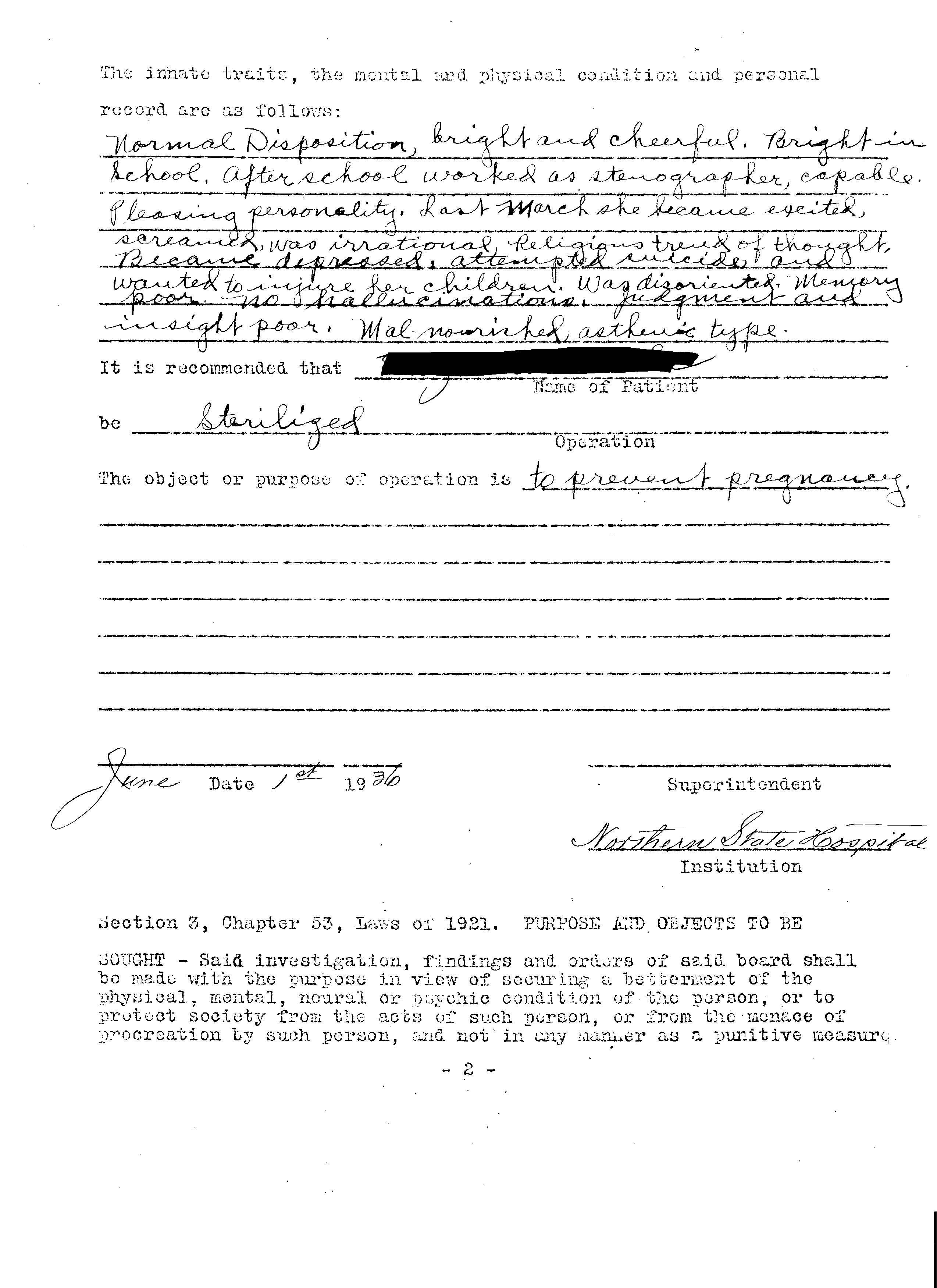
Thirty states adopted legislation to perform forced sterilization on those deemed “mentally unfit.”
The burden of the “feebleminded”
“It is a reproach to our intelligence that we as a people should have to support about half a million insane, feebleminded, epileptic, blind and deaf; 80,000 prisoners and 100,000 paupers at a cost of over 100 million dollars per year.”
-Charles Davenport, founder of the Eugenics Record Office, 1910
Compulsory segregation and sterilization
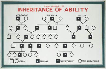
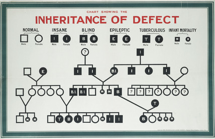
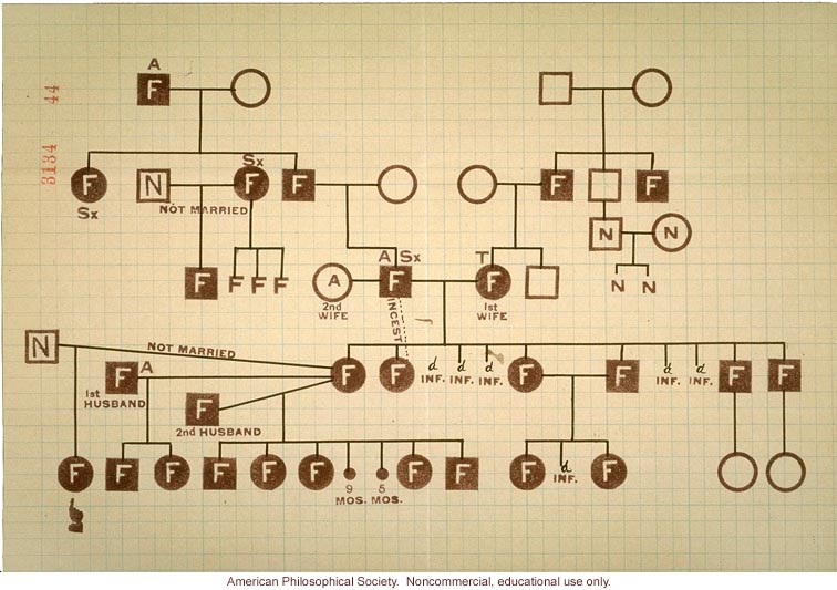
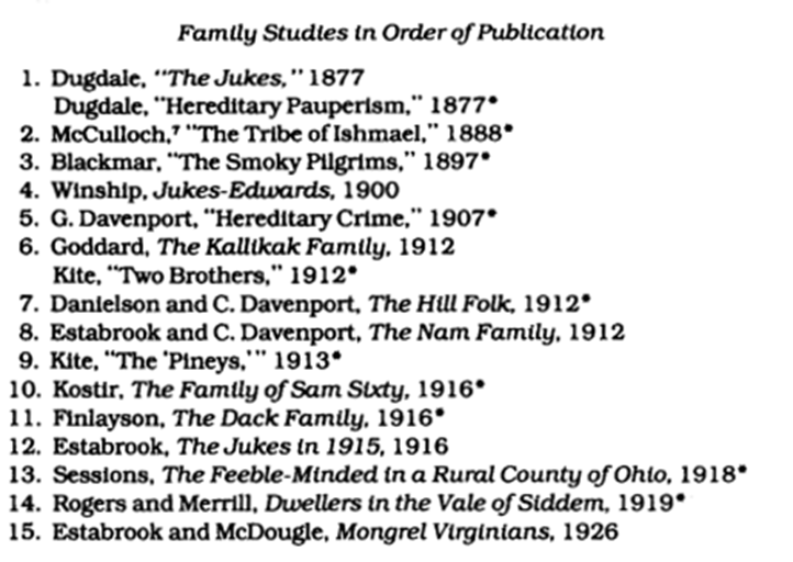
Eugenics Record Office pedigree showing transmission of feeblemindedness over several generations. Such evidence supported state-mandated, coerced sterilization of at least 62,000 Americans in over 30 states, beginning in 1907.
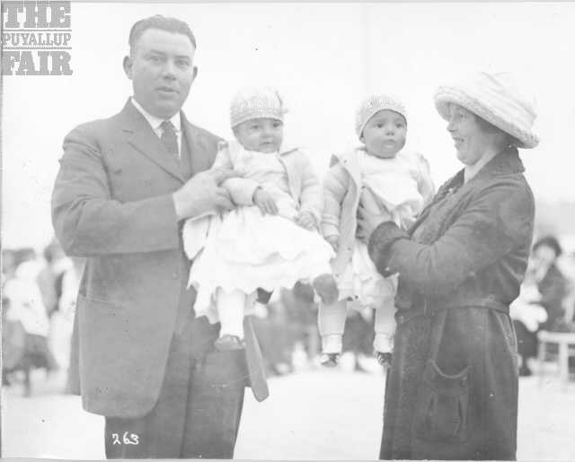
Better Babies at the Puyallup Fair, 1910s
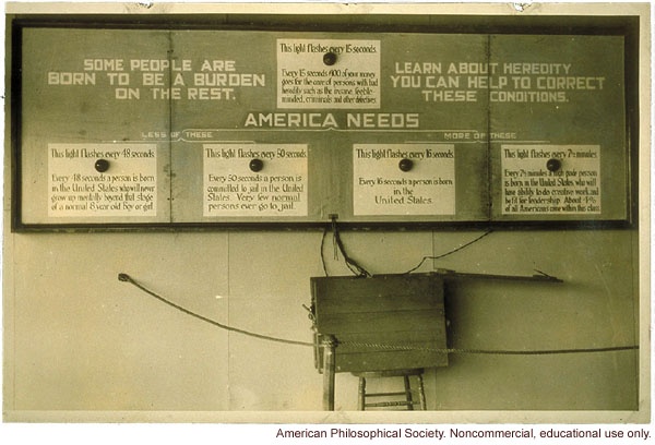
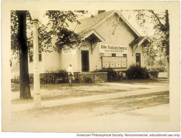
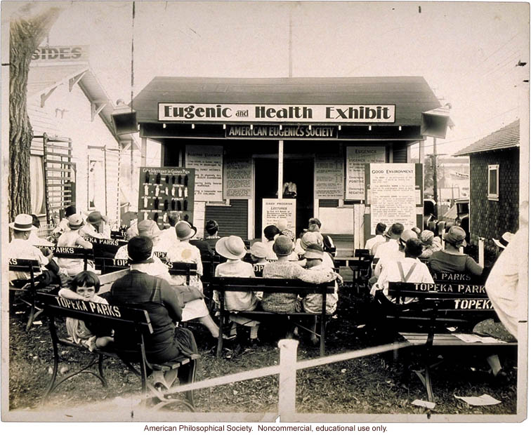
Positive eugenics: Fitter Families contests and educational exhibits
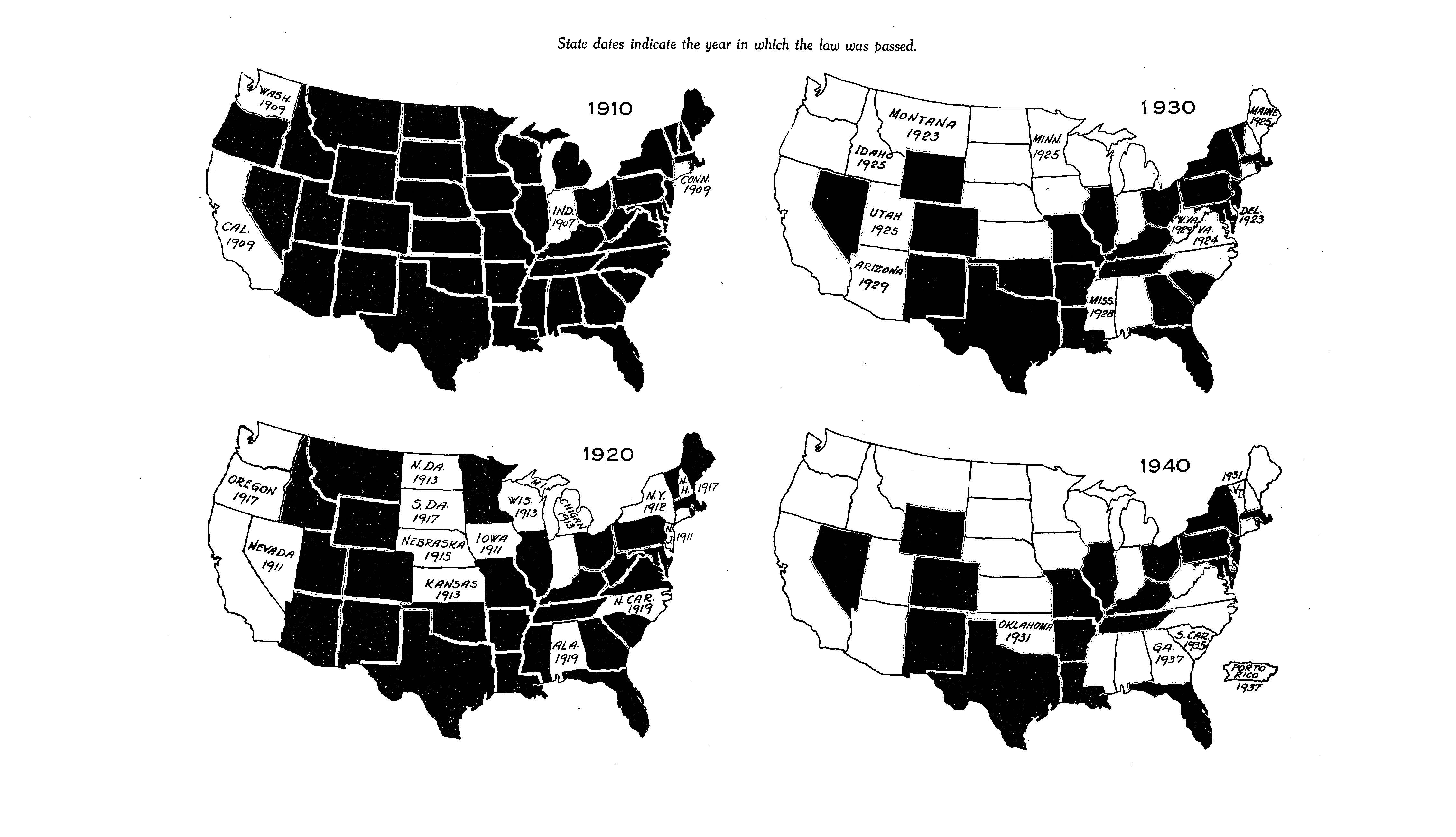
Sterilization Laws in the US
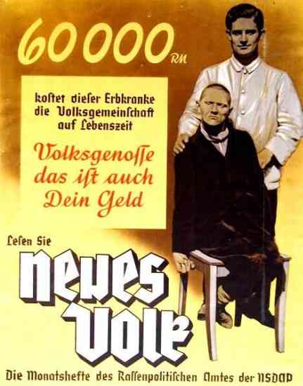
Why Nazi Germany stands out
Importance of ideology of national fitness and purity to politics and culture: ‘the ’racial state’
Leader in psychiatric and genetic science
Opportunities from a sympathetic state
Degree of economic problems via depression and mobilisation of economy in WWII
Scale of sterilisation policy (375,000)
Use of ‘euthanasia’ for mentally handicapped (Action T4 – 70,000)
Yet German eugenics has roots before Nazi era
Sterilisation Law introduced before Nazis come to power
Follows example of USA
Eugenics and an interest in ‘race hygiene’ well established (1st society 1905)
Germany already a leader in eugenic sciences of psychiatry and genetics, e.g. via Kaiser Wilhelm Institute (and has financial support from Rockefeller Foundation into 1930s)
Deaths of mentally ill in German asylums in First World War (140,000)
U.S. (and Canada)
Nazi Germany
Period
1907-late 1970s
1934-1945
Total
70,000
375,000 (= approx. 1% of adult population of childbearing age) + 70,000 killed
Disproportionately targeted
Disabled; also disenfranchised, poor, women, minorities
Same
Law
State
Federal
Compulsion
Typically formally voluntary (required formal consent)
Compulsory
Reach
Mostly only institutionalized (in a few cases, “extra mural”)
Everyone
Text of the law
Varied across states; basic elements similar
Similar to H. Laughlin’s model sterilization law
Adjudication
Typically eugenics boards; proceedings public; victims could challenge in civil court
Special “hereditary health courts”; non-public; appeal only to superior health courts
Denunciation by general public (information to commence sterilization proceedings)
No
Yes
Authorities’ access to medical and other records of kin groups
Could be extensive
Extensive
The post-war reckoning
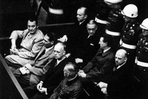
At post-war Nazi trials the question of medical experiments is subject for prosecution, but eugenics itself in fact attracts little attention
Not until 1970s and 1980s and a new generation of historians does it come into focus
After the second World War
Eugenics is scientifically and culturally discredited
It disappears from Universities and the public discourse
But sterilizations continue in US and Scandinavia (Sweden) till the 70s
% female victims
% mentally ill
% intellectually disabled
total
victims per year / 100,000 pop. in peak period
sterilization period (length of time)
National
61%
44%
52%
Est. 70,000+
1907-earl.1980s (75 years)
CA
49%
58%
37%
20,000
13
1909-60s (55 years)
MN
78%
18%
82%
2,300
5
1925-earl.1960s (35 years)
VA
61%
49%
48%
7,300
13
1924-1979s (50 years)
IA
71%
44%
50%
1,910
6
1915-earl.1960s (35 years)
GA
55%
77%
22%
3,200
9
1937-1963 (25 years)
NC
83%
25%
70%
6,300
7
1929-1974 (45 years)
% female victims
% mentally ill
% intellectually disabled
NC
83%
25%
70%
NC targeted “black welfare queens” in 1950s and 1960s; sterilization law had “extra-mural” component and allowed sterilization of populations not in state institutions
% female victims
% mentally ill
% intellectually disabled
MN
78%
18%
82%
MN: strength of social progressivism with a focus on ‘helping’ intellectually disabled females; sterilization of insane required at least 6 months of continuous institutionalization and consent by individual and next of kin
Eugenics as a Pseudoscience
Made-up categories
One encompassing explanation (interpretation Vs explanation)
“It is unmitigated humbug to talk about hereditary class distinctions being rooted in Nature. An individual is, of course, a product of nature and nurture, but it is one-tenth the former and nine-tenths the latter”
Today?
Abortion is legal for serious fetal anomaly
To prevent life-long suffering for the affected
Euthanasia (for the terminally ill) is illegal but, to some extent, tolerated
COVID-19
Where do we draw a line?
Midterm
Midterm Thursday during class time
Exam: 40 questions total + formula sheet + z-table
A few questions are worth more than one point
Problems: boxplots, contingency table, z-scores, regression, probability
Best way to study: review HW and class exercises
Review lectures slides
Final grades will be curved
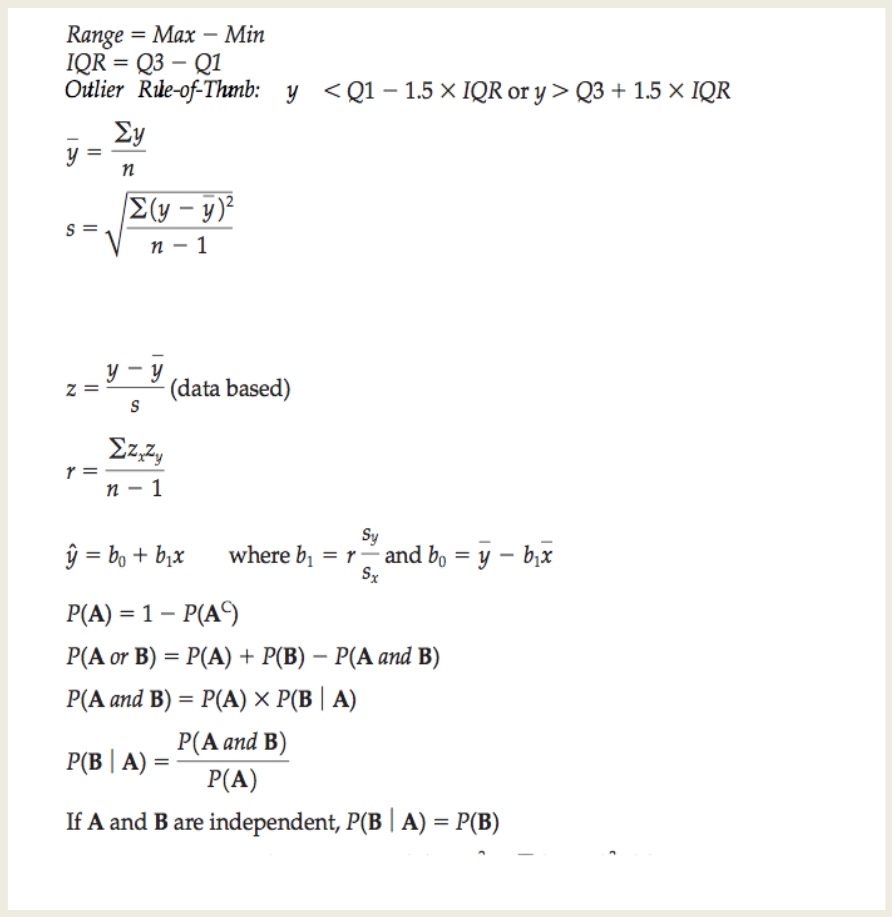
Formula sheet
Chapter 1
Introduction
Why do we need statistics?
Statistics helps us make sense of the data and how the data vary.
Statistics is about variation.
Statistics is a collection of conceptual and mathematical tools that allow us to study such variation.
Why is Statistics important for Psychology?
The use of Statistics qualifies Psychology as a science…
using statistics we can determine whether a psychological hypothesis is true for a wider population, or whether a treatment works or not.
Statistical methods provide a unifying force within Psychology.
Data
Data
Any collection of numbers, characters, images, or other items that provide information about something
Data vary: Surveys and experiments produce a variety of outcomes.
Statistical inference is making a decision or a conclusion based on the data.
Sample and Population
The goal is to describe the population.
This is usually impractical or impossible.
A sample is used to make inferences about the population.
The sample should be representative of the population.
Variables
Categorical Variable: A variable that tells us what group or category an individual belongs to
Quantitative Variable: Contains measured numerical values with measurement units
Identifier Variable: A variable that is used to uniquely identify the individual. It does not describe the individual.
Ordinal Variable: A variable that reports order without natural units
Chapter 2
Displaying and Describing Categorical Data
How to Display Categorical Data
How to display and describe categorical data
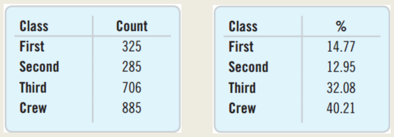
Frequency tables
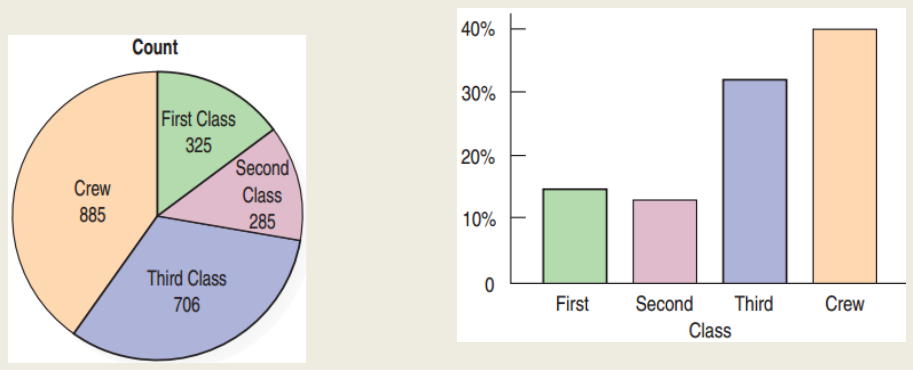
Bar Charts
Pie Charts
Comparing Categorical Data
How to compare categorical data:
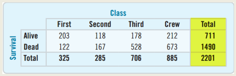
Contingency tables
Marginal distribution
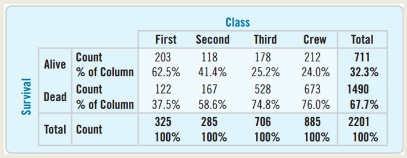
Conditional distribution:
percent of one variable satisfying the conditions of another
can be organized by column or by row
Independence
Independence: The distribution of one variable is the same for all categories of another.
There is no association between the two.
An association that holds for all of several groups can reverse direction when the data are combined to form a single group. This reversal is called Simpson’s paradox.
Chapter 3
Displaying and Summarizing Quantitative Data
Display of Quantitative Data: Histograms
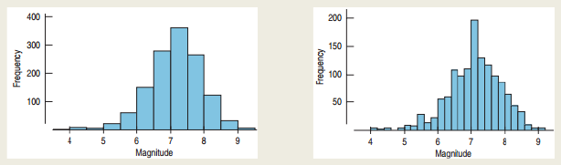
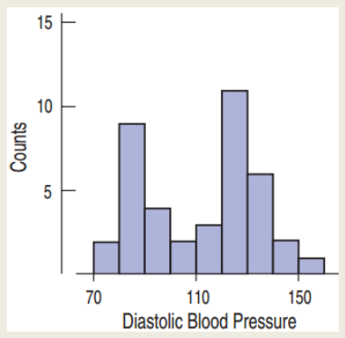
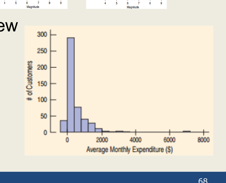
How to display quantitative data: histograms
bin width
shape: mode, symmetry, skew
outliers
Display of Quantitative Data: Histograms
How to display quantitative data: histograms
CENTER: median, mean
Median: the center of data values
not sensitive to outliers
Mean: average
sensitive to outliers
\[\bar{y} = \frac{\sum y}{n}\]
Outliers
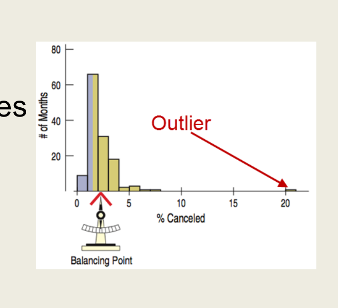
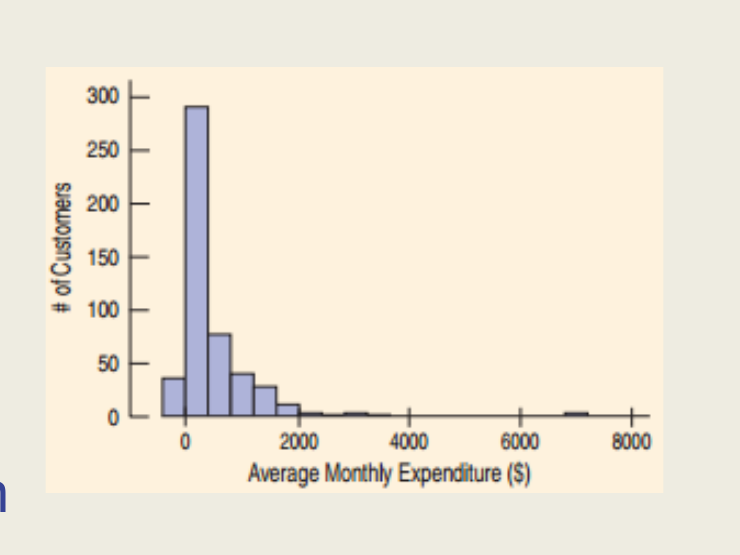
An Outlier is a data value that is far above or far below the rest of the data values.
An outlier is sometimes just an error in the data collection.
An outlier can also be the most important data value.
Income of a CEO
Temperature of a person with a high fever
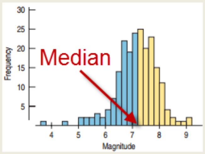
Center: the Median
Median: The center of the data values
Half of the data values are to the left of the median and half are to the right of the median.
For symmetric distributions, the median is directly in the middle.
Calculating the Median: Odd Sample Size
First order the numbers.
If there are an odd number of numbers, n, the median is at position \(\frac{n+1}{2}\).
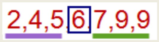
Find the median of the numbers: 2, 4, 5, 6, 7, 9, 9.
\(\frac{n+1}{2} = \frac{7+1}{2} = 4\)
The median is the fourth number: 6
Note that there are 3 numbers to the left of 6 and 3 to the right.
Calculating the Median: Even Sample Size
First order the numbers.
If there are an even number of numbers, n, the median is the average of the two middle numbers: \(\frac{n}{2}, \frac{n}{2}+1\).
Find the median of the numbers: 2, 2, 4, 6, 7, 8.
\(\frac{n}{2} = \frac{6}{2} = 3\)
The median is the average of the third and the fourth numbers:
\[\text{Median} = \frac{4+6}{2} = 5\]
The Center of Symmetric Distributions: the Mean
The Mean is what most people think of as the average.
Add up all the numbers and divide by the number of numbers.
\[\bar{y} = \frac{\sum y}{n}\]
Recall that \(\sum\) means “Add them all.”
Mean Vs. Median
For symmetric distributions, the mean and the median are equal.
The balancing point is at the center.
The tail “pulls” the mean towards it more than it does to the median.
The mean is more sensitive to outliers than the median.
Spread
SPREAD: variance, standard deviation
The variance is a measure of how far the data is spread out from the mean.
The standard deviation is the square root of the variance
The sd expresses the average distance from the mean
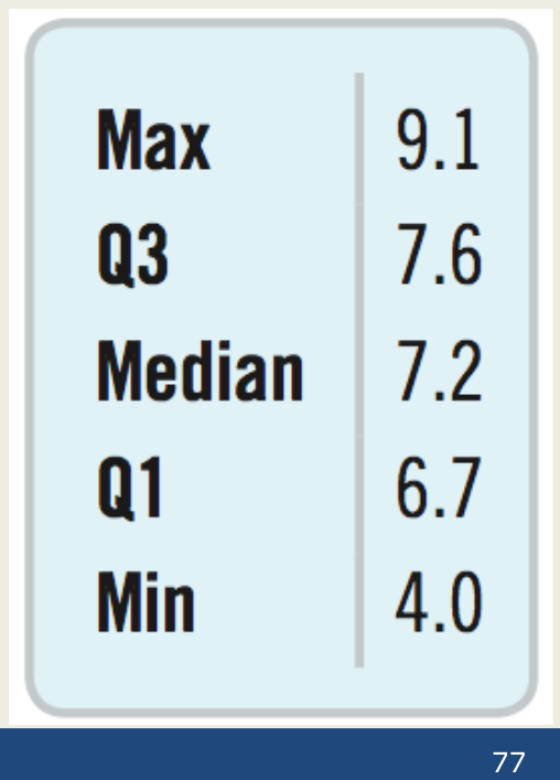
The 5-Number Summary provides a numerical description of the data. It consists of
Minimum
First Quartile (Q1)
Median
Third Quartile (Q3)
Maximum
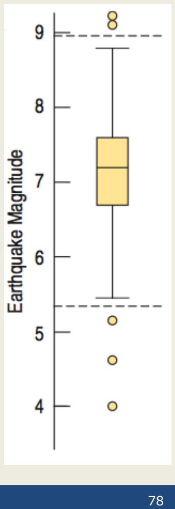
The list to the right shows the 5-Number Summary for the tsunami data.
Boxplots
A Boxplot is a chart that displays the 5-Point Summary and the outliers.
The Box shows the Interquartile Range.
The dashed lines are called fences, outside the fences lie the outliers.
Above and below the box are the whiskers that display the most extreme data values within the fences.
The line inside the box shows the median.
Finding the Fences
The lower fence is defined by
Lower Fence = Q1 – 1.5 × IQR
The upper fence is defined by
Upper Fence = Q3 + 1.5 × IQR
Chapter 4
Understanding and Comparing Distributions
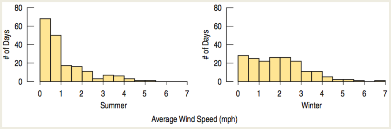
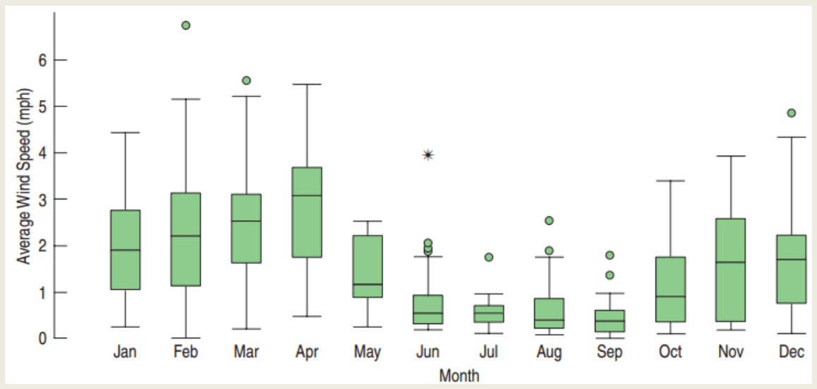
How to compare quantitative data
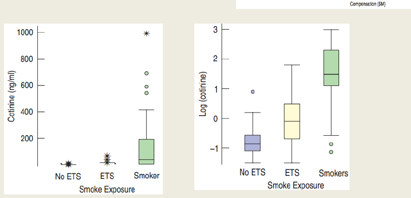
How to compare quantitative data: histograms and boxplots
How to compare quantitative data
How to compare quantitative data: histograms and boxplots
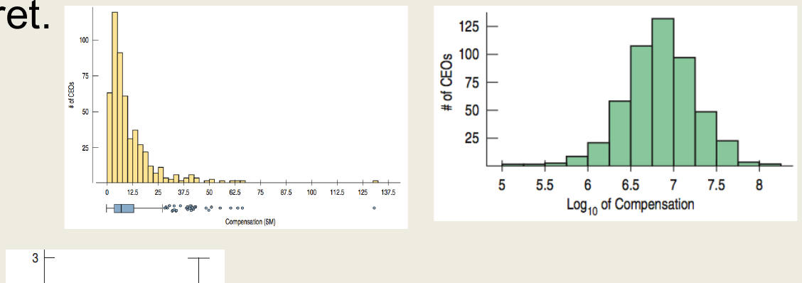
Transformation of the Data
Taking logarithm of the salaries makes histogram much easier to interpret.
Chapter 5
The Standard Deviation as a Ruler and the Normal Model
How Many Standard Deviations From the Mean?
The standard deviation helps us compare: how far from the mean?
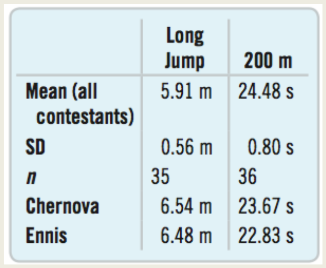
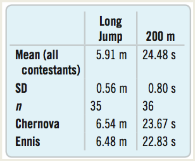
Chernova’s long jump was more than 1 standard deviation better than the mean.
Ennis’s winning time in the 200 m was more than 2 standard deviations faster than the mean.
Is there an even more precise way to calculate these?
The z-Score
In general, to find the distance between the value and the mean in standard deviations:
Subtract the mean from the value.
Divide by the standard deviation.
\[z = \frac{y - \bar{y}}{s}\]
This is called the z-score.
The z-score
The z-score measures the distance of the value from the mean in standard deviations.
A positive z-score indicates the value is above the mean.
A negative z-score indicates the value is below the mean.
A small z-score indicates the value is close to the mean when compared to the rest of the data values.
A large z-score indicates the value is far from the mean when compared to the rest of the data values.
How Many SDs from Mean?
Chernova’s long jump
\[z = \frac{6.54 - 5.91}{0.56} \approx 1.1\]
Ennis’s 200 m run
\[z = \frac{22.83 - 24.48}{0.80} \approx -2.1\]
Ennis’s winning time is a little more impressive.
Judges could assign points based on standard deviations from mean and this system would have a correlation of 0.99 with the one currently used!
How Many SDs from Mean?
\(-1 < z < 1\): Not uncommon
\(z = \pm 3\): Rare
\(z = 6\): Shouts out for attention!
Shifting
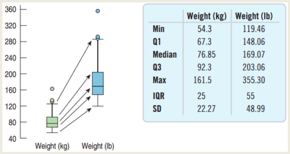
If the same number is subtracted or added to all data values, then:
The measures of the spread – standard deviation, range, and IQR – are all unaffected.
The measures of position – mean, median, and mode – are all changed by that number.
Rescaling
When we multiply (or divide) all the data values by a constant, all measures of position and all measures of spread are multiplied (or divided) by that same constant.