Quantitative Methods

Lecture 11

Serena DeStefani

2020-07-27

Quantitative Methods

Serena DeStefani – Lecture 11 – 7/27/2020

How did we get here?

• Statistics is about variation, specifically in data
• Types of variables
• How to represent variables
  • bar graphs
  • boxplots, histograms
• How to compare apples and oranges
  • by their variation (z scores)
  • are they varying together? correlation and regression

How did we get here?

• Statistics is about variation, specifically in data
• What am I interested in?
• A larger group, or population
• How to get data?
• Surveys
• Impossible to survey the population
• → representative sample (SRS)
• But exactly what does the population think?
• What’s the population parameter?
• Experiments
• Is my result due to the treatment or is it due to chance?

How did we get here?

• Two questions:
  • What’s the population parameter?
  • Is my result likely?
• To answer these questions I need a probability model
• The rules of probability
• Random variable: the Bernoulli trial
• The geometric and binomial distribution
• The normal approximation to the binomial
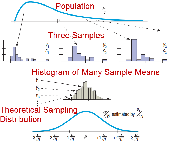
• The sampling distribution
• The Central Limit Theorem

Sampling About Climate Change

According to a Gallup poll of 1022 Americans, 57% believe that climate change is due to human activity.

• If many surveys were done of 1022 Americans, we could calculate the sample proportion for each.

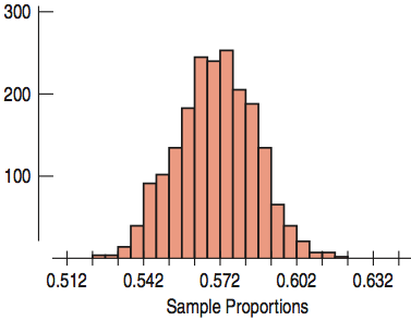
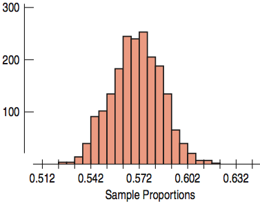
• The histogram shows the distribution of a simulation of 2000 sample proportions.
• The distribution of all possible sample proportions from samples with the same sample size is called the sampling distribution.

Sampling Distributions for Proportions

Sampling Distribution for Proportions

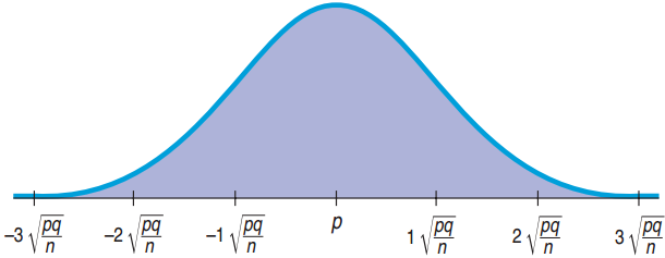
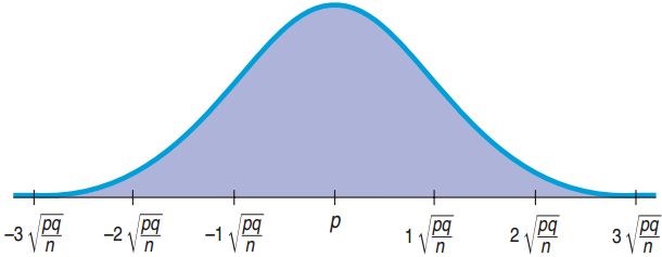
• Symmetric
• Unimodal
• Centered at p
• The sampling distribution follows the Normal model.

What does the sampling distribution tell us?

• The sampling distribution allows us to make statements about where we think the corresponding population parameter is and how precise these statements are likely to be.

From One Sample to Many Samples

Distribution of One Sample

• Variable was the answer to the survey question or the result of an experiment.
• Proportion is a fixed value that comes from the one sample.

Sampling Distribution

• Variable is the proportion that comes from the entire sample.
• Many proportions that differ from one to another, each coming from a different sample.

Mean and Standard Deviation

Sampling Distribution for Proportions

• \(\text{Mean} = p\)
• \(\sigma(\hat{p}) = \dfrac{\sqrt{npq}}{n} = \sqrt{\dfrac{pq}{n}}\)
• \(N\left(p, \sqrt{\dfrac{pq}{n}}\right)\)

This p is a parameter!

Instead \(\hat{p}\) is a statistic!

The Normal Model for Climate Change

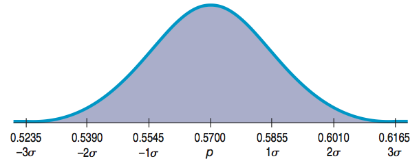
Population: p = 0.57, n = 1022. Sampling Distribution:

• Mean = 0.57
• Standard deviation \(= SD(\hat{p}) = \sqrt{\dfrac{(0.57)(0.43)}{1022}} \approx 0.0155\)

Standard Error

The sample-to-sample standard deviation is called the standard error or sampling variability.

• The standard error is not a “real” error, since no error has been made.

The problem is, we don’t know the population parameter.

Sampling Distributions for Means

How did we get here?

• What’s the population parameter?
  • → Confidence Intervals
• Is my result likely?
  • → Hypothesis testing

Where are we going?

• Confidence intervals
• Hypothesis testing for proportions
• Hypothesis testing for means
• What if I have more than two groups?

Chapter 18

Confidence Intervals for Proportions

18.1

A Confidence Interval

Mean and Standard Deviation

Sampling Distribution for Proportions

• \(\text{Mean} = p\)
• \(\sigma(\hat{p}) = \dfrac{\sqrt{npq}}{n} = \sqrt{\dfrac{pq}{n}}\)
• \(N\left(p, \sqrt{\dfrac{pq}{n}}\right)\)

Standard Deviation for a Proportion?

What is the sampling distribution?

• Usually we do not know the population proportion p.
• We cannot find the standard deviation of the sampling distribution: \(\sqrt{\dfrac{pq}{n}}\)
• After taking a sample, we only know the sample proportion, which we use as an approximation.
• The sample-to-sample standard deviation is called the standard error or sampling variability
• The standard error is given by \(SE(\hat{p}) = \sqrt{\dfrac{\hat{p}\hat{q}}{n}}\)

Facebook Daily Status Updates

A recent survey found that 48 of 156 or 30.8% update their Facebook status daily.

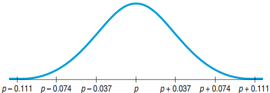
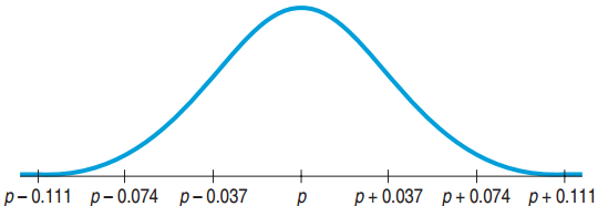
\[SE(\hat{p}) = \sqrt{\frac{\hat{p}\hat{q}}{n}} = \sqrt{\frac{(0.308)(0.692)}{156}} \approx 0.037\]

• The sampling distribution is approximately normal.

Facebook: true population proportion?

A recent survey found that 48 of 156 or 30.8% update their Facebook status daily.

• This is the sample proportion
• What is the true population proportion?
• To find it, we need to make an inference using the sampling distribution we just found, based on SE

Interpreting this Normal Curve

• By normality, about 95% of all possible samples of 156 young Facebook users will have \(\hat{p}\)’s within 2 SE (0.037) of p
• If \(\hat{p}\) is close to p, then p is close to \(\hat{p}\).
• If you stand at \(\hat{p}\), then you can be 95% sure that p is within 2 SE’s from where you are standing.
• → Our confidence interval: (0.234, 0.382)

What You Can Say About p if You Know \(\hat{p}\)

We don’t know exactly what percent of all Facebook users update their status daily, but the interval from 23.4% to 38.2% probably contains the true proportion.

• Note, we admit we are unsure about both the exact proportion and whether it is in the interval.

We are 95% confident that between 23.4% and 38.2% of all Facebook users update their status daily.

• Notice “% confident” and an interval rather than an exact value are stated.

What You Cannot Say About p if You Know \(\hat{p}\)

30.8% of all Facebook users update their status daily.

• We can’t make such absolute statements about p.

It is probably true that 30.8% of all Facebook users update their status daily.

• We still cannot commit to a specific value for p, only a range.

We don’t know exactly what percent of all Facebook users update their status daily, but we know it is within the interval 30.8% ± 2 × 3.7%.

• We cannot be certain it is in this interval.

Naming the Confidence Interval

This confidence interval is a one-proportion z-interval.

• “One” since there is a single survey question.
• “Proportion” since we are interested in the proportion of Facebook users who update their status daily.
• “z-interval” since the distribution is approximately normal.

18.2

Interpreting Confidence Intervals: What Does 95% Confidence Really Mean?

Capturing a Proportion

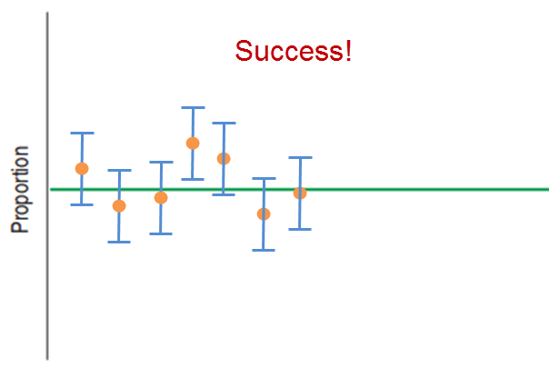
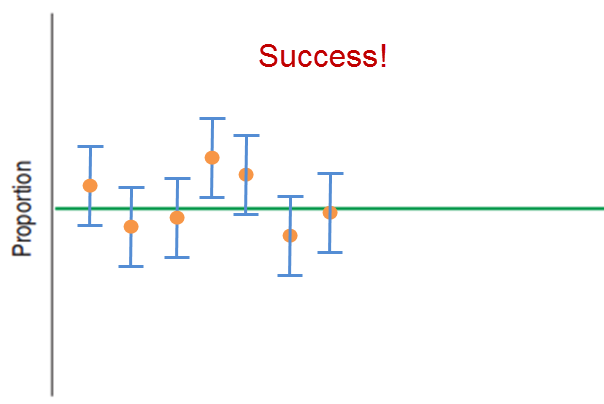
• The confidence interval may or may not contain the true population proportion.
• Consider repeating the study over and over again, each time with the same sample size.
  • Each time we would get a different \(\hat{p}\).
  • From each \(\hat{p}\), a different confidence interval could be computed.
  • About 95% of these confidence intervals will capture the true proportion.
  • 5% will not.

Simulating Confidence Intervals

Confidence Intervals

There are a huge number of confidence intervals that could be drawn.

• In theory, all the confidence intervals could be listed.
• 95% will “work” (capture the true proportion).
• 5% will not capture the true proportion.

What about our confidence interval (0.234, 0.382)?

• We will never know whether it captures the population proportion.

“Statistics Means Never Having to Say You Are Certain”

Facebook Status Updates

Technically Correct

• I am 95% confident that the interval from 23.4% to 38.2% captures the true proportion of Facebook users who update daily.

More Casual But Fine

• I am 95% confident that between 23.4% and 38.2% of Facebook users update daily.

18.3

Margin of Error: Certainty vs. Precision

Margin of Error

• Confidence interval for a population proportion (95%):

\[\hat{p} \pm 2SE\left(\hat{p}\right)\]

• The distance, \(2SE\left(\hat{p}\right)\), from \(\hat{p}\) is called the margin of error.
• Confidence intervals also work for means, regression slopes, and others. In general, the confidence interval has the form

\[\text{Estimate} \pm ME\]

Simulating Confidence Intervals

Certainty vs. Precision

• Instead of a 95% confidence interval, any percent can be used.
• Increasing the confidence (e.g. 99%) increases the margin of error.
• Decreasing the confidence (e.g. 90%) decreases the margin of error.

Confidence Interval on Global Warming

Yale and George Mason University interviewed 1010 US adults about beliefs and attitudes on global warming. They presented a 95% confidence interval on the proportion who think there is disagreement among scientists.

• Had the polling been done repeatedly, 95% of all random samples would yield confidence intervals that contain the true population proportion of all US adults who believe there is disagreement among scientists.

Yale/George Mason Study Revisited

The poll of 1010 adults reported a margin of error of 3%. (by convention, 95% with “worst case” ME based on p = 0.5)

• How was the 3% computed?

\[SE(\hat{p}) = \sqrt{\frac{(0.5)(0.5)}{1010}} \approx 0.0157\]

• For 95% confidence: \(ME = 2(0.0157) = 0.031\)
• The margin of error is close to 3%.

Critical Values

• For a 95% confidence interval, the margin of error was 2SE.
  • The 2 comes from the normal curve.
  • 95% of the area is within about 2SE from the mean.
• In general the number of SE is called the critical value. Since we use the normal distribution here we denote it \(z^*\)
• To be more precise, \(z^*\) for 95% CI is 1.96

Finding the Critical Value

Find the critical value corresponding to 90% confidence.

• 90% inside gives 10% outside.
• 2 tails outside with 10% means 1 tail with 5% or 0.05.
• The critical value is about \(z^* = 1.645\).

Finding the Margin of Error (Take 2)

Yale/George Mason Poll: 1010 US adults, 40% think scientists disagree about global warming. At 95% confidence ME = 3%.

• Find the margin of error at 90% confidence.

Finding the Margin of Error (Take 2)

Yale/George Mason Poll: 1010 US adults, 40% think scientists disagree about global warming. At 95% confidence ME = 3%.

• Find the margin of error at 90% confidence.

\[SE(\hat{p}) = \sqrt{\frac{(0.4)(0.6)}{1010}} \approx 0.0154\]

• For 90%, \(z^* \approx 1.645\): \(ME = (1.645)(0.0154) = 0.025\).
• This gives a smaller margin of error which is good.
• Drawback: lower level of confidence which is bad

18.4

Assumptions and Conditions

Independence and Sample Size

• Independence Condition
  • If data is collected using SRS or a randomized experiment → Randomization Condition
  • Some data values do not influence others.
  • Check for the 10% Condition: The sample size is less than 10% of the population size.
• Success/Failure Condition
  • There must be at least 10 successes.
  • There must be at least 10 failures.

One-Proportion z-Interval

• First check for randomization, independence, 10%, and conditions on sample size.
• Confidence level C, sample size n, proportion \(\hat{p}\).
• Confidence interval: \(\hat{p} \pm z^{*}SE\left(\hat{p}\right)\)
• \(SE\left(\hat{p}\right) = \sqrt{\dfrac{(\hat{p})(\hat{q})}{n}}\)
• \(z^*\): the critical value that specifies the number of SE’s needed for C% of random samples to yield confidence intervals that capture the population proportion.

Do You Believe the Death Penalty is Applied Fairly?

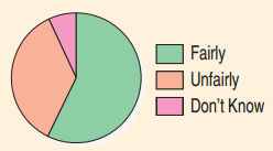
• Sample size: 510
• Answers:
  • 58% “Fairly”
  • 36% “Unfairly”
  • 7% “Don’t Know”
• Construct a confidence interval for the population proportion that would reply “Fairly.”

Do You Believe the Death Penalty is Applied Fairly?

• Plan: Find a 95% confidence interval for the population proportion.
• Model:
  • Randomization: Randomly selected by Gallup Poll
  • 10% Condition: Population is all Americans
  • Success/Failure Condition
    • (510)(0.58) = 296 ≥ 10, (510)(0.42) = 214 ≥ 10
  • Use the Normal Model to find a one-proportion z-interval.

Do You Believe the Death Penalty is Applied Fairly?

• Mechanics: n = 510, \(\hat{p} = 0.58\)

Do You Believe the Death Penalty is Applied Fairly?

• Mechanics: n = 510, \(\hat{p} = 0.58\)

\[SE(\hat{p}) = \sqrt{\frac{(0.58)(0.42)}{510}} \approx 0.022\]

• \(z^* \approx 1.96\)
• \(ME \approx (1.96)(0.022) \approx 0.043\)
• The 95% Confidence Interval is: 0.58 ± 0.043 or (0.537, 0.623)

Do You Believe the Death Penalty is Applied Fairly?

• Conclusion: I am 95% confident that between 53.7% and 62.3% of all US adults think that the death penalty is applied fairly.

What Sample Size?

\[ME = z^* \sqrt{\frac{\hat{p}\hat{q}}{n}}\]

• For example, to ensure a ME < 3%:
• For 95%, \(z^* = 1.96\)

What Sample Size?

\[ME = z^* \sqrt{\frac{\hat{p}\hat{q}}{n}}\]

• For example, to ensure a ME < 3%:
• For 95%, \(z^* = 1.96\)
• Values that make ME largest are \(\hat{p} = 0.5,\ \hat{q} = 0.5\)

\[0.03 = 1.96\sqrt{\frac{(0.5)(0.5)}{n}}\]

• Solving for n, gives n ≈ 1067.1.
• We need to survey at least 1068 to ensure a ME less than 0.03 for the 95% confidence interval.

The Yale/George Mason Survey and Sample Size

Poll: 40% believe scientists disagree on global warming.

• For a follow-up survey, what sample size is needed to obtain a 95% confidence interval with ME ≤ 2%?

\[ME = z^* \sqrt{\frac{\hat{p}\hat{q}}{n}}\]

The Yale/George Mason Survey and Sample Size

Poll: 40% believe scientists disagree on global warming.

• For a follow-up survey, what sample size is needed to obtain a 95% confidence interval with ME ≤ 2%?

\[ME = z^* \sqrt{\frac{\hat{p}\hat{q}}{n}} \qquad 0.02 = 1.96\sqrt{\frac{(0.4)(0.6)}{n}}\]

• n ≈ 2304.96
• The group will need at least 2305 respondents.

Thoughts on Sample Size and ME

• Obtaining a large sample size can be expensive and/or take a long time.
• For a pilot study, ME = 10% can be acceptable.
• For full studies, ME ≤ 5% is better.
• Public opinion polls typically use ME = 3%, n = 1000.
• If p is expected to be very small such as 0.005, then much smaller ME such as 0.1% is required.

Credit Cards and Sample Size

A pilot study showed that 0.5% of credit card offers in the mail end up with the person signing up.

• To be within 0.1% of the true rate with 95% confidence, how big does the test mailing have to be?

\[ME = z^* \sqrt{\frac{\hat{p}\hat{q}}{n}}\]

Credit Cards and Sample Size

A pilot study showed that 0.5% of credit card offers in the mail end up with the person signing up.

• To be within 0.1% of the true rate with 95% confidence, how big does the test mailing have to be?

\[ME = z^* \sqrt{\frac{\hat{p}\hat{q}}{n}} \qquad 0.001 = 1.96\sqrt{\frac{(0.005)(0.995)}{n}}\]

• n ≈ 19,111.96
• The test mailing should include at least 19,112 offers.

What Can Go Wrong?

Don’t claim other samples will agree with yours.

• Wrong: In 95% of samples, between 43% and 51% agree with decriminalization of marijuana.

Don’t be certain about the parameter.

• Wrong: Between 23% and 38% of Facebook users update daily. Don’t forget to include the confidence.

Don’t forget that it’s about the parameter (not the statistics)

• Wrong: I’m 95% confident that \(\hat{p}\) is between 23% and 38%. You know for sure exactly what \(\hat{p}\) is.

What Can Go Wrong?

Don’t claim to know too much.

• Wrong: I’m 95% confident that between 23% and 38% of all Facebook users in the world update daily. The survey was just about US residents between 18 and 22.

Do take responsibility.

• Accept that you are only 95% confident, not sure.

Don’t suggest that the parameter varies… it does not!

• Wrong: There is a 95% chance that the true parameter is between 23% and 38%.

What Can Go Wrong?

Do treat the whole interval equally.

• The middle of the interval is not necessarily more plausible than the edges.

Beware of margins of error that are too large to be useful.

• Between 10% and 90% update daily is not useful. Use a larger sample size to shrink the ME.

Watch out for biased sampling.

• Biased samples produce unreliable CIs.

Think about independence

• Be careful in your sample design to ensure randomization.

Chapter 19

Testing Hypotheses About Proportions

19.1

Hypotheses

Cracking Rate < 20%?

General cracking rate: 20%

After a new engineering process, the cracking rate of 400 casts fell to 17%!

Is this due to the new engineering or just random chance?

• Null Hypothesis (\(H_0\)): Nothing has changed
  • \(H_0\): proportion = hypothesized value
  • \(H_0\): p = 0.20
• Alternative Hypothesis:
  • \(H_A\): p < 0.20

How Small to Convince Us?

• Had the new cracking rate been 1%, it would clearly indicate a change from 20%.
  • Extremely unlikely that this could happen just by random chance
• Had the new cracking rate been 19.8%, we would be skeptical.
  • Not so unlikely to be just random chance
• How about 17%?
  • How likely is it that a random sample would have a cracking rate 17% or less?

Checking Conditions and Finding the Standard Error

Checking Conditions: n = 400, p = 0.20

• np = (400)(0.20) = 80 ≥ 10
• nq = (400)(0.80) = 320 ≥ 10
• Independence plausible
• The Normal model applies.

Find the standard deviation of the model.

\[SD(\hat{p}) = \sqrt{\frac{pq}{n}} = \sqrt{\frac{(0.20)(0.80)}{400}} = 0.02\]

• Note: Use p and not \(\hat{p}\) to find standard deviation.

Using the Normal Model

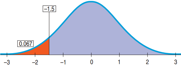
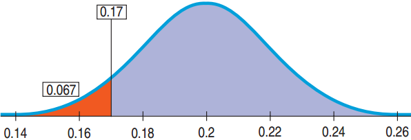
p = 0.20, \(\hat{p}\) = 0.17, \(SD(\hat{p})\) = 0.02

Using the Normal Model

p = 0.20, \(\hat{p}\) = 0.17, \(SD(\hat{p})\) = 0.02

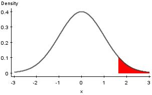
\[z = \frac{0.17 - 0.20}{0.02} = -1.5\]

\[P(z < -1.5) \approx 0.067\]

• If the null hypothesis is true that the cracking rate is still equal to 20%, then the probability of observing a cracking rate of 17% in a random sample of 400 is 6.7%.

Innocent until Proven Guilty

• Begin with the presumption of innocence (\(H_0\)).
• Collect evidence.
  • Bank money in house
  • Still wearing mask
  • Getaway car found in his name
• Evidence beyond a reasonable doubt?
  • Is 5% small enough chance?
  • How about 1%?
  • 6.7%?

19.2

P-Values

The P-Value and Surprise

The P-value is the probability of seeing data like these (or even more unlikely-extreme data) given the null hypothesis is true.

• Tells us how surprised we would be to get these data given \(H_0\) is true.
  • P-value small: Either \(H_0\) is not true or something remarkable occurred
  • P-value not small enough: Not a surprise. Data consistent with the model. Do not reject \(H_0\).

Guilty or Not Enough Evidence?

Defendant is either

• Guilty: P-value too small. The evidence is clear.
• Not Guilty: P-value not small enough. The evidence is not sufficient. Not the same as innocent. Maybe innocent or maybe guilty, but not enough evidence found.

Two Choices

• Fail to reject \(H_0\) if P-value large. Never accept \(H_0\).
• Reject \(H_0\) if P-value is small. Accept \(H_A\).

When the P-Value is Not Small

Wrong

• Accept \(H_0\).
• We have proven \(H_0\).

Right

• Fail to reject \(H_0\)
• There is insufficient evidence to reject \(H_0\).
• \(H_0\) may or may not be true.

Example: \(H_0\): All swans are white.

• If we sample 100 swans that are all white, there could still be a black swan.

19.3

The Reasoning of Hypothesis Testing

Step 1: State the Hypotheses

\(H_0\):

• \(H_0\) usually states that there’s nothing different.
• \(H_0\): parameter = hypothesized value
• Note the parameter describes the population not the sample.
• \(H_0\) is called the null hypothesis.

\(H_A\):

• \(H_A\) is a statement that something has changed, gotten bigger or smaller
• \(H_A\) is called the alternative hypothesis.

Hypotheses About the DMV

The DMV claims 80% of all drivers pass the driving test. In a survey of 90 teens, only 61 passed.

• Is there evidence that teen pass rates are below 80%?
  • \(H_0\): p = 0.80
  • \(H_A\): p < 0.80

Step 2: Model

Decide on the model to test the null hypothesis and parameter.

• Check conditions, e.g. independence, sample size.
• If the conditions are not met, either quit or redesign the study.
• Normal models use z-scores. Other models may not use z-scores.
• Name the model, e.g. 1-proportion z-test.

1-Proportion z-Test

Conditions

• Same as a 1-Proportion z-Interval

Null Hypothesis

• \(H_0\): \(p = p_0\)

Test Statistics

\[z = \frac{\hat{p} - p_0}{SD\left(\hat{p}\right)} \qquad SD\left(\hat{p}\right) = \sqrt{\frac{p_0 q_0}{n}}\]

DMV Study: Checking Conditions

• Randomization Condition: The 90 teens were a random sample of all teens.
• 10% Condition: 90 is fewer than 10% of the total number of all teens who take the driving test.
• Success/Failure Condition:
  • \(np_0\) = (90)(0.80) = 72 ≥ 10
  • \(nq_0\) = (90)(0.20) = 18 ≥ 10
• The conditions are satisfied. We can use the Normal model and perform a 1-Proportion z-Test.

DMV Study: Mechanics

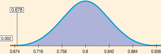
Claim: 80% pass. 61 of 90 teens tested passed.

• Find P-value.
  • n = 90, x = 61, \(p_0\) = 0.80, \(\hat{p} = \dfrac{61}{90} \approx 0.678\)

DMV Study: Mechanics

Claim: 80% pass. 61 of 90 teens tested passed.

• Find P-value.
  • n = 90, x = 61, \(p_0\) = 0.80, \(\hat{p} = \dfrac{61}{90} \approx 0.678\)

\[SD(\hat{p}) = \sqrt{\frac{p_0 q_0}{n}} \approx \sqrt{\frac{(0.80)(0.20)}{90}} \approx 0.042\]

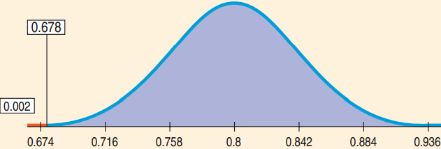
\[z = \frac{0.678 - 0.80}{0.042} \approx -2.90\]

\[\text{P-value} = P(z < -2.90) \approx 0.002\]

DMV Study: Conclusion

Is the teen pass rate less than 80%? P-value = 0.002

• What can be concluded? What does the P-value mean?
  • P-value = 0.002 is very small → Reject \(H_0\)
  • The survey data provide strong evidence that the pass rate for teens is less than 80%.
  • This should not be the end of the conversation.
  • The next step would be to see if the pass rate is low enough to take further action.

19.4

Alternative Alternatives

Two-Sided Alternative

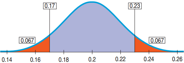
For the new process the engineer may be interested in whether there has been a change in the cracking rate not just a decrease.

• \(H_0\): p = 0.20
• \(H_A\): p ≠ 0.20

• An alternative hypothesis where we are interested in deviation on either side is called a two-sided alternative.
• The P-value is the probability of deviating from either direction from the null hypothesis.

One-Sided Alternative

The engineer may be interested in whether there has been a decrease in the cracking rate.

• \(H_0\): p = 0.20
• \(H_A\): p < 0.20

• An alternative hypothesis where we are interested in deviation on only one side is called a one-sided alternative.
• The P-value for a one-sided alternative is always half the P-value for the two-sided alternative.

Not the Right Proportion of Male Babies?

Under natural conditions, 51.7% of births are male. In Punjab India’s hospital 56.9% of the 550 births were male.

• Question: Is there evidence that the proportion of male births is different for this hospital?
• Plan: We will have a two-tailed alternative. The parameter of interest is p.
  • \(H_0\): p = 0.517
  • \(H_A\): p ≠ 0.517

Not the Right Proportion of Male Babies?

• Model: Check the conditions
  • Independence Assumption: The sex of one baby should not affect the sex of others.
  • Randomization Conditions: The births were not random, so be cautious of the results.
  • 10% Condition: 550 births is certainly less than the total number of all births.

Not the Right Proportion of Male Babies?

• Model: Check the conditions (Continued).
  • Success/Fail Condition: (550)(0.517) ≥ 10, (550)(0.483) ≥ 10
  • The Normal model does apply.
  • We can use a one-proportion z-test.

Not the Right Proportion of Male Babies?

• Mechanics:

\[SD(\hat{p}) = \sqrt{\frac{p_0 q_0}{n}} \approx \sqrt{\frac{(0.517)(1-0.517)}{550}} \approx 0.0213\]

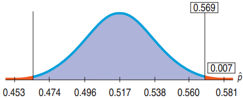
\[z = \frac{\hat{p} - p_0}{SD\left(\hat{p}\right)} = \frac{0.569 - 0.517}{0.0213} \approx 2.44\]

Not the Right Proportion of Male Babies?

Show →

• Mechanics:

\[\text{P-value} = 2P(z > 2.44) = 2(0.0073) = 0.0146\]

Not the Right Proportion of Male Babies?

• Conclusion:
  • Interpreting the P-value = 0.0146
    • If the proportion of male babies were still 51.7%, then an observed proportion as different as 56.9% male babies would occur at random about 15 times in 1000.
    • This is so small a chance that I reject \(H_0\). There is strong evidence that the proportion of boys is not equal to the baseline for the region. It appears larger.

19.5

P-Values and Decisions: What to Tell About a Hypothesis Test

How Small a P-Value is Small Enough?

How small is small enough is context specific.

• Test to see if a renowned musicologist can distinguish between Mozart and Haydn.
  • P-value of 0.1 may be good enough. Just reaffirming known talent.
• A friend claims psychic abilities and can predict heads or tails.
  • Very small P-value such as 0.01 needed. Breaking scientific theory.

Acceptable P-Value Depends on Result’s Importance

Proportion of students in school with full time jobs has increased.

• Not that important. P-value = 0.05 will work.

Testing the proportion of faulty rivets that hold together the wings of a commercial aircraft is now below the danger threshold.

• Life and death decision. Need a very small P-value
• Whether rejecting or failing to reject, always cite the P-value.
• An accompanying confidence interval helps also.

Home Field Advantage?

Is there a home field advantage in baseball?

• The home team won 1308 of the 2431 (53.81%) games played in the season.
• Is there evidence to suggest that the home team wins more than 50%?
• Plan: p = proportion of home team wins
• Hypotheses
  • \(H_0\): p = 0.50
  • \(H_A\): p > 0.50

Home Field Advantage?

Model →

• Independence Assumption: Questionable, but the 2013 season may be representative of all games past and future.
• 10% Condition: The 2013 season is less than 10% of all games played past and future.
• Success/Failure Condition:
  • np = (2431)(0.5) ≥ 10
  • nq = (2431)(0.5) ≥ 10
• The Normal Model Applies: Conduct a one-proportion z-test.

Home Field Advantage?

• Mechanics:

\[SD(\hat{p}) = \sqrt{\frac{p_0 q_0}{n}} \approx \sqrt{\frac{(0.5)(1-0.5)}{2431}} \approx 0.010141\]

\[z = \frac{\hat{p} - p_0}{SD\left(\hat{p}\right)} = \frac{0.53805 - 0.5}{0.010141} \approx 3.75\]

• The P-value is about 0.0001.

Home Field Advantage?

• Conclusion: The P-value of 0.0001 says that if the true proportion of home team wins is 0.5 then an observed value of 0.53805 would occur less than 1 time in 1000.
• This is so unlikely, so reject \(H_0\).
• There is reasonable evidence that the true proportion of home team wins is greater than 50%.
• There appears to be a home field advantage.

How Big a Home Field Advantage?

• Model:
  • Success Failure Condition (notice difference!)
    • Home team wins: 1308 ≥ 10
    • Home team losses: 1123 ≥ 10
  • Sampling distribution follows the Normal model.
  • Find the one-proportion z-interval.

How Big a Home Field Advantage?

• Mechanics (notice difference!):

\[SE(\hat{p}) = \sqrt{\frac{\hat{p}\hat{q}}{n}} \approx \sqrt{\frac{(0.53805)(1-0.53805)}{2431}} \approx 0.01011\]

• For 95% confidence, \(z^* = 1.96\).

\[ME = z^* \times SE(\hat{p}) = 1.96 \times 0.01011 = 0.0198\]

• A 95% confidence interval is: 0.53805 ± 0.0198 or (0.5182, 0.5579).

How Big a Home Field Advantage?

Tell →

• Conclusion: I am 95% confident that, in professional baseball, home teams win between 51.82% and 55.79% of the games.
• For a 162-game season, the low end gives the home team about 1/2 of an extra victory and the high end, about 4 extra wins.

What Can Go Wrong?

Don’t base your \(H_0\) on what you see in the data.

• Changing the null hypothesis after looking at the data is just wrong.

Don’t base your \(H_A\) on the data.

• Both the null and alternative hypotheses must be stated before peeking at the data.

Don’t make \(H_0\) what you want to show to be true.

• \(H_0\) represents the status quo. You can never accept the null hypothesis.

What Can Go Wrong?

Don’t forget to check the conditions.

• Randomization, independence, and sample size

Don’t accept the null hypothesis.

• You can only say you don’t have evidence to reject \(H_0\) (you can only say you “fail to reject”).

If you fail to reject \(H_0\) don’t expect a larger sample would reject \(H_0\).

• Check the confidence interval. If its values would not matter to you, then a larger sample will unlikely be worthwhile.