Quantitative Methods

Lecture 13

Serena DeStefani

2020-07-29

Quantitative Methods

Serena DeStefani – Lecture 13 – 7/29/2020

Announcements

• Midterm overview tomorrow
• HW 6 due tomorrow
• R2 assignment due on Sunday
• HW 7 due on Tuesday

Review of key terms

• \(s\)   \(\sigma\)
  • The standard deviation of the sample
  • The standard deviation of the population
• \(SD(\hat{p})\)   \(SE(\hat{p})\)
  • The standard deviation of the sampling distribution for a proportion
  • The standard error: an approximation calculated from the sample proportion
• \(SD(\bar{y})\)   \(SE(\bar{y})\)
  • The standard deviation of the sampling distribution for a mean
  • The standard error: an approximation calculated from the sample mean

Review: Inference about means

The Central Limit Theorem (CLT)

When a random sample is drawn from a population with mean \(\mu\) and standard deviation \(\sigma\), the sampling distribution has a normal shape with:

• Mean: \(\mu\)
• Standard deviation SD: \(\dfrac{\sigma}{\sqrt{n}}\)
• → we can use the normal model to make inference for means, as we did for proportions.
• Problem: the sampling distribution is approximately normal as long as the sample size is large.
• What if sample size is small?

Review: Gosset at Guinness

At Guinness, Gosset experimented with beer.

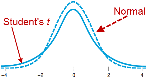
• The Normal Model was not right, especially for small samples.
• Still bell shaped, but details differed, depending on n
• Came up with the “Student’s t Distribution” as the correct model

Review: Sampling distribution for Means

• For every sample size n there is a different Student’s t distribution.
• Degrees of freedom: df = n – 1.

Sampling Distribution Model for Means

\[t = \frac{\bar{y} - \mu}{SE(\bar{y})} \qquad SE(\bar{y}) = \frac{s}{\sqrt{n}}\]

Review: One Sample t-Interval for the Mean

• When the assumptions are met (seen later), the confidence interval for the mean is

\[\bar{y} \ \pm \ t^{*}_{n-1} \times SE(\bar{y})\]

• The critical value \(t^{*}_{n-1}\) depends on the confidence level, C, and the degrees of freedom n – 1.

Review: How Much Sleep do College Students Get?

Build a 90% Confidence Interval for the Mean.

• Plan: Data on 25 Students

Model →

• Randomization Condition The data are from a random survey.
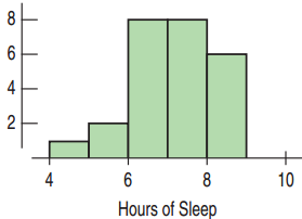
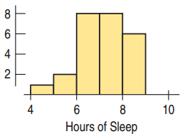
• Nearly Normal Condition Unimodal and slightly skewed, so OK
• Use Student’s t-Model with df = 25 – 1 = 24.
• One-sample t-interval for the mean

How Much Sleep?

• Mechanics: n = 25, \(\bar{y}\) = 6.64, s = 1.075
  • Remember, when we calculate a CI for means, we get t* (a.k.a. the critical value) from a computer or a table. When we perform a hypothesis test, we compute t directly.
  • The steps are: calculate SE, get t*, calculate ME and then the interval

How Much Sleep?

• Mechanics: n = 25, \(\bar{y}\) = 6.64, s = 1.075

\[SE(\bar{y}) = \frac{s}{\sqrt{n}} = \frac{1.075}{\sqrt{25}} = 0.215 \text{ hours}\]

\[t^{*}_{24} = 1.711\]

\[\begin{align} ME &= t^{*}_{24} \times SE(\bar{y}) \\ &= 1.711 \times 0.215 \\ &= 0.368 \text{ hours} \end{align}\]

\[90\% \text{ CI} = 6.64 \pm 0.368 = (6.272, 7.008)\]

How Much Sleep do College Students Get?

• Conclusion: I’m 90 percent confident that the interval from 6.272 and 7.008 hours contains the true population mean number of hours that college students sleep.

Do Students Get at Least Seven Hours of Sleep? 25 Surveyed.

• Plan: Is the mean amount of sleep less than 7 hours?
• Hypotheses: \(H_0\): \(\mu = 7\)   \(H_A\): \(\mu < 7\)
• Model
  • Randomization Condition: The students were randomly and independently selected.
  • Nearly Normal Condition: Unimodal and symmetric
  • Use the Student’s t-model, df = 24
  • One-sample t-test for the mean

Do Students Get at Least Seven Hours of Sleep? 25 Surveyed.

• Mechanics: n = 25, \(\bar{y}\) = 6.64, s = 1.075, \(\mu\) = 7
• This is an hypothesis test! To perform it, we calculate t directly.

Do Students Get at Least Seven Hours of Sleep? 25 Surveyed.

• Mechanics: n = 25, \(\bar{y}\) = 6.64, s = 1.075

\[SE(\bar{y}) = \frac{s}{\sqrt{n}} = \frac{1.075}{\sqrt{25}} = 0.215 \text{ hours}\]

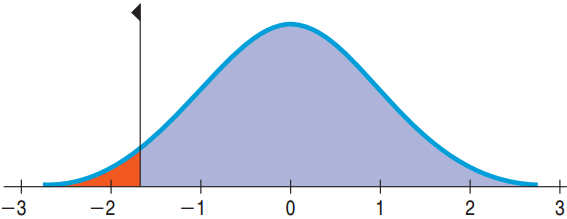
\[t = \frac{\bar{y} - \mu_0}{SE(\bar{y})} = \frac{6.64 - 7.0}{0.215} \approx -1.67\]

\[\text{P-value} = P(t_{24} < -1.67) \approx 0.054\]

Or between 0.05 and 0.10 using the t-table

Do Students Get at Least Seven Hours of Sleep? 25 Surveyed.

• Conclusion: P-value = 0.054 says that if students do sleep an average of 7 hrs. (= if a model of the sampling distribution centered at 7 hrs. is the correct one) samples of 25 students can be expected to have an observed mean of 6.64 hrs. or less about 54 times in 1000.
• With 0.05 cutoff, there is not quite enough evidence to conclude that the mean sleep is less than 7.

Do Students Get at Least Seven Hours of Sleep? 25 Surveyed.

• With 0.05 cutoff, there is not quite enough evidence to conclude that the mean sleep is less than 7.
• We have seen there is correspondence between HT and CI
• This result can also be inferred from the CI
• The 90% CI built on our sample mean: (6.272, 7.008) contains 7.
• That means the sample mean is not distant enough from the hypothesized mean of the sampling dist. (7)
• Collecting a larger sample would reduce the ME and give us a better handle on the true mean hours of sleep.

Do Students Get at Least Seven Hours of Sleep? 25 Surveyed.

• Remember, the SE depends on the sample size!
• The larger the sample size, the smaller the SE
• The smaller the SE:
  • The bigger t is – result more likely to be significant
  • The smaller ME is – the smaller CI is – the less likely the CI to contain the hypothesized mean of the sampling distribution (\(H_0\))
• Collecting a larger sample would reduce the ME and give us a better handle on the true mean hours of sleep.

Do Students Get at Least Seven Hours of Sleep? 25 Surveyed.

• Collecting a larger sample would reduce the ME and give us a better handle on the true mean hours of sleep.
• But if the sample is big enough, any result will be significant!
• You have to decide: is the difference big enough?

Intervals and Tests

Confidence Intervals

• Start with data and find plausible values for the parameter.
• Always 2-sided

Hypothesis Tests

• Start with a proposed parameter value and then use the data to see if that value is not plausible.

What Can Go Wrong?

Don’t confuse proportions and means.

• When counting successes with a proportion, use the Normal model
  • → for HT of sample vs. population, use SD calculated from population proportion
  • → for CI of population proportion, use SE calculated from sample proportion
• With means and small samples, use Student’s t.
  • → use SE calculated from sample mean s

What Can Go Wrong?

Beware of multimodality.

• If the histogram is not unimodal, consider separating into groups and analyzing each group separately.

Beware of skewed data.

• Look at the normal probability plot and histogram.
• Consider re-expressing if the data is skewed.

What Can Go Wrong?

Set outliers aside.

• Outliers violate the Nearly Normal Condition.
• If removing a data value substantially changes the conclusions, then you have an outlier.
• Analyze without the outliers, but be sure to include a separate discussion about the outliers.

Watch out for bias.

• With bias, even a large sample size will not save you.

What Can Go Wrong?

Make sure cases are independent.

• Look for violations of the independence assumption.

Make sure the data are from an appropriately randomized sample.

• Without randomization, both the confidence interval and the p-value are suspect.

Interpret your confidence interval correctly.

• The CI is about the mean of the population, not the mean of the sample, individuals in samples, or individuals in the population (but you use it SE!)

Chapter 21

More About Tests and Intervals

21.1

Choosing Hypotheses

Choosing the Null

The null hypothesis typically means no change or no difference.

• Identify the status quo or value that indicates that things are the same.
• This does not mean 0. \(H_0\): p = 0 is rarely correct.
• The null hypothesis is never shown to be true.

The alternative hypothesis is that things did decrease, increase or change.

• It’s what you are interested in showing is true.

Examples of Choosing Hypotheses

The helmet law was dropped for those over 21. You are interested in whether people under 21 are now less likely to wear a helmet. Before dropping the law 60% of youths wore helmets.

• \(H_0\): p = 0.6
• \(H_A\): p < 0.6

Have athletes’ strength increased with the new exercise equipment?

• \(H_0\): \(\mu\) = past mean strength
• \(H_A\): \(\mu\) > past mean strength

Hypotheses for Avandia

There is concern about the Type 2 diabetes drug Avandia raising the risk of heart attack. People with Type 2 diabetes have a 20.2% chance of heart attack within 7 years. 28.9% of the 4485 people with Type 2 diabetes had heart attacks within 7 years.

• What are the null and alternative hypotheses?
  • \(H_0\): p = 0.202
  • \(H_A\): p > 0.202
• We use a one-sided upper-tailed test since we are concerned about a higher risk of heart attack.

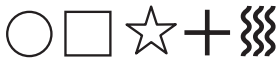
Are You Psychic?

The test is to use your psychic abilities to determine which symbol the person is concentrating on. If you are psychic, you should do better than 20%.

• \(H_0\): p = 0.20   \(H_A\): p > 0.20

But maybe there is interference, so performing lower than 20% would also indicate ESP.

• \(H_0\): p = 0.20   \(H_A\): p ≠ 0.20

21.2

How to Think about P-Values

P-Value is a Conditional Probability

The P-value is the probability of getting results as unusual as observed given that \(H_0\) is true.

• P-value = P(observed stat value | \(H_0\) is true)
• P-value ≠ P(\(H_0\) is true | observed stat value)

The P-value never gives a probability that \(H_0\) is true.

• P-value = 0.03 does not mean a 3% chance of \(H_0\) being correct.
• It just says that if \(H_0\) is correct, then there would be a 3% chance of observing a statistic value more unlike the null value.

Small P-Values

A smaller P-value provides stronger evidence against \(H_0\).

• This does not mean that \(H_0\) is less true.
• The person is not more guilty, you just are more convinced of the guilt.

There is no hard and fast rule on how small is small enough.

• How believable is \(H_0\)?
• Do you trust your data?

Has Helmet Use Declined among Youth Since the Law Changed?

• Plan: The proportion before was 60%. Now I run a study on 781 subjects. 396 were wearing helmets, or 50.7%. Is this evidence that the proportion has declined, or is this a random fluctuation?
• Hypotheses: The status quo is that the proportion of youth wearing helmets is still 60%. We are interested in whether this proportion has declined.
  • \(H_0\): p = 0.60
  • \(H_A\): p < 0.60

Has Helmet Use Declined among Youth Since the Law Changed?

• Model:
  • Independence Assumption: The accident victims were independent of each other.
  • Randomization Condition: Great effort was taken to make the sample representative.
  • Success/Failure Condition:
    • \(np = (781)(0.6) = 468.6 \geq 10\)
    • \(nq = (781)(0.4) = 312.4 \geq 10\)
  • Use the Normal model and a one-proportion z-test.

Has Helmet Use Declined among Youth Since the Law Changed?

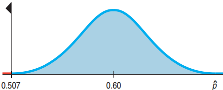
N=781, 396 wearing helmets, p=60%

Has Helmet Use Declined among Youth Since the Law Changed?

N=781, 396 wearing helmets, p=60%

• Mechanics:

\[\hat{p} = \frac{396}{781} \approx 0.507\]

\[SD(\hat{p}) = \sqrt{\frac{p_0 q_0}{n}} = \sqrt{\frac{(0.6)(0.4)}{781}} \approx 0.0175\]

\[z = \frac{\hat{p} - p_0}{SD(\hat{p})} = \frac{0.507 - 0.60}{0.0175} \approx -5.31\]

• P-value < 0.001

Has Helmet Use Declined among Youth Since the Law Changed?

• Conclusion: The very small p-value tells us that if helmet rate among youth were still 60%, then there would be less than a 1 in 1000 chance of observing a rate no higher than 50.7%.
• Reject \(H_0\).
• There is strong evidence that there has been a decline in helmet use among riders under 21.

How Much Has Helmet Use Declined?

• The strong evidence for a decline does not mean a large decline.
• Instead use a confidence interval.

How Much Has Helmet Use Declined?

• The strong evidence for a decline does not mean a large decline.
• Instead use a confidence interval.

\[\hat{p} \pm z^{*}\sqrt{\frac{\hat{p}\hat{q}}{n}} = 0.507 \pm 1.96(0.0175) = (0.472, 0.542)\]

• With 95% confidence, helmet use declined between 6% and 13%.

P-value Expresses Evidence Against the Null

A Bank Robbery Trial:

1. The getaway car’s color matches the defendant’s.
   • P-value pretty large
2. Both robber and defendant have same color hair and same height and weight.
   • P-value getting smaller
3. Robber’s jacket found in trash near defendant’s house.
   • P-value still smaller

Diabetes Drug Revisited

The sample of patients who took the drug had 28.9% heart attack risk while the general population has a 20.2% risk.

• Interpret the P-value.

\[\text{P-value} = P(\hat{p} \geq 28.9\% \mid p = 20.2\%)\]

• The P-value represents the probability of seeing such a high heart attack rate among those studied if, in fact, taking the drug doesn’t increase risk at all.

Detecting the Human Energy Field

The Therapeutic Touch (TT) practitioners tried to decide whether the girl’s hand hovered over the left or right hand.

Detecting the Human Energy Field

The Therapeutic Touch (TT) practitioners tried to decide whether the girl’s hand hovered over the left or right hand.

• \(H_0\): p = 0.5   \(H_A\): p > 0.5
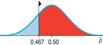
• TT practitioners successful 70 of 150 tries: \(\hat{p} = 46.7\%\)

Detecting the Human Energy Field

The Therapeutic Touch (TT) practitioners tried to decide whether the girl’s hand hovered over the left or right hand.

• \(H_0\): p = 0.5   \(H_A\): p > 0.5
• TT practitioners successful 70 of 150 tries: \(\hat{p} = 46.7\%\)

\[SD(\hat{p}) = \sqrt{\frac{(0.5)(0.5)}{150}} \approx 0.041, \quad z = \frac{0.467 - 0.5}{0.041} = -0.805\]

\[P(z > -0.805) = 0.790\]

How to Interpret P-Value = 0.790

• The P-value of 0.790 is so large we certainly do not reject \(H_0\).
• P-value > 0.5 indicates that the sample was on the wrong side of the inequality.
• The TT practitioners were worse not better than random chance alone.
• This does not mean the null hypothesis is true, only that we cannot say it is false.

More on P-Values

An earlier study on the risk of the diabetes drug reported an increased risk of heart attack from 20.2% to 26.9% and a P-value of 0.27.

• Why did the researchers not express alarm?
• P-value = 0.27 means that there would be a 27% chance of at least such an increase for a sample even if there were no increased risk for the drug.

21.3

Alpha Levels

How to Define “Rare Enough”

• Need to make a decision whether P-value is low enough to reject \(H_0\).
• → Set a threshold value
• This is called the alpha level (\(\alpha\)).
• P-value < \(\alpha\):
  • Reject \(H_0\).
  • The results are statistically significant.
• P-value > \(\alpha\):
  • Fail to reject \(H_0\).
  • The results are not statistically significant.

Choosing an \(\alpha\)

• \(\alpha\) = 0.05 is most common
  • (1 in 20 chances is pretty rare)
• Other levels of significance commonly used:
  • 0.001, 0.01, 0.1
• Are the air bags safe?
  • Low \(\alpha\) such as 0.001.
• Do students like pepperoni or sausage?
  • High \(\alpha\) such as 0.1.

Just Make a Decision

The level of significance forces us to make a decision.

• P-Value below \(\alpha\):
  • “The test is significant at that level.”
• P-Value above \(\alpha\):
  • “The data have failed to provide sufficient evidence to reject the null hypothesis.”
  • We “fail to reject” \(H_0\).
  • → Never “accept” \(H_0\).
• Always include the actual P-value.
  • Showing the P-value is far below \(\alpha\) tells a different story than when the P-value is just below \(\alpha\).

Practical vs. Statistical Significance

Practical Significance

• The results noticeably differ from the status quo.
  • Proportion of wins = 85% vs. the expected 50%.
  • Mean exam score 48 without studying vs. the course mean of 82.

Statistical Significance

• P-value < \(\alpha\)
• If the status quo is true, it would be unlikely for a sample to have such extreme mean or proportion.

Are They Speeding?

• College Terrace speed limit: 25 mph
• Even after traffic-calming measures, a resident complains that cars still speed.
• 250 of 2000 randomly selected cars were clocked with mean speed 25.55 mph, s = 3.618.
• Is the mean speed of all cars greater than 25 mph?
  • \(H_0\): \(\mu\) = 25
  • \(H_A\): \(\mu\) > 25

Are They Speeding?

• Independence Assumption:
  • The random sample makes the independence assumption reasonable.
  • The 10% condition is close enough to being met.
• Nearly Normal Condition
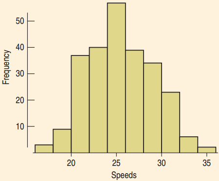
  • The histogram is unimodal and symmetric. There are no outliers. The sample size is large.

Are They Speeding?

• n = 250, df = 249, \(\bar{y}\) = 25.55, s = 3.618, \(\mu\) = 25

Are They Speeding?

• n = 250, df = 249, \(\bar{y}\) = 25.55, s = 3.618

\[SE(\bar{y}) = \frac{3.618}{\sqrt{250}} \approx 0.2288\]

\[t_{249} = \frac{25.55 - 25}{0.2288} \approx 2.404\]

\[P(t_{249} > 2.404) = 0.0085\]

or P between 0.01 and 0.005 from the table, P<0.01

• A 95% confidence interval is (25.099, 26.001).

Are They Speeding?

• P-value = 0.0085 is very small.
• Reject the null hypothesis and conclude that the mean speed is greater than 25 mph.
• This is statistically significant but is it practically significant?
• Is 25.55 mph noticeably faster than 25 mph?
• Even at the high end of the CI, 26 mph, should the City Council make an effort based on this finding?

21.4

Critical Values for Hypothesis Tests

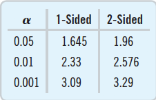
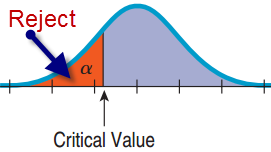
Critical Values: An Alternative to P-Values (before we had computers)

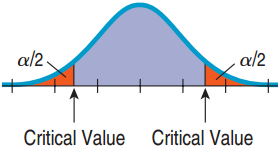
• For a hypothesis test look at the z-axis (or t-axis) to decide on whether to reject \(H_0\).
• Find the value of z (or t) that corresponds to \(\alpha\).

• 2-tails: use \(\alpha/2\)

Critical Values vs. P-Values

• Critical values give a value of z or t to compare with the test statistic in order to determine statistical significance.
• The P-value is compared with \(\alpha\) to determine statistical significance.
• The P-value is richer. It also has meaning as a probability.

Confidence Intervals and Hypothesis Tests

• A confidence interval contains all plausible values.
• Two Tailed Test: Value outside, null hypothesis rejected. \(\alpha\) = 100 – C.
  • C = 95% → \(\alpha\) = 5%
• One Sided Test: \(\alpha\) = ½ (100 – C)
  • C = 95% → \(\alpha\) = ½(100 – 95) = 2.5%
  • A one-sided test at 5% corresponds to a 90% CI

Decisions from a Confidence Interval

There is concern about the Type 2 diabetes drug Avandia raising the risk of heart attack. People with Type 2 diabetes have a 20.2% chance of heart attack within 7 years. 28.9% of the 4485 people with Type 2 diabetes had heart attacks within 7 years.

The 95% CI for the proportion of those who took the drug that had heart attacks was 20.8% to 40.0%

• What can you say about the drug’s safety?
  • 20.2 < 20.8
  • There is evidence of an increased risk.

Decisions from a Confidence Interval

There is concern about the Type 2 diabetes drug Avandia raising the risk of heart attack. People with Type 2 diabetes have a 20.2% chance of heart attack within 7 years. 28.9% of the 4485 people with Type 2 diabetes had heart attacks within 7 years.

The 95% CI for the proportion of those who took the drug that had heart attacks was 20.8% to 40.0%

• What can you say about the drug’s safety?
  • 20.2 < 20.8
  • There is evidence of an increased risk.

Decisions from a Confidence Interval

There is concern about the Type 2 diabetes drug Avandia raising the risk of heart attack. People with Type 2 diabetes have a 20.2% chance of heart attack within 7 years. 28.9% of the 4485 people with Type 2 diabetes had heart attacks within 7 years.

The 95% CI for the proportion of those who took the drug that had heart attacks was 20.8% to 40.0%

• What can you say about the drug’s safety?
  • 20.2 < 20.8
  • There is evidence of an increased risk.

Decisions from a Confidence Interval

There is concern about the Type 2 diabetes drug Avandia raising the risk of heart attack. People with Type 2 diabetes have a 20.2% chance of heart attack within 7 years. 28.9% of the 4485 people with Type 2 diabetes had heart attacks within 7 years. Hypothesis test?

The 95% CI for the proportion of those who took the drug that had heart attacks was 20.8% to 40.0% Confidence interval?

• What can you say about the drug’s safety?
  • 20.2 < 20.8
  • There is evidence of an increased risk.

21.5

Errors

Type I and II Errors

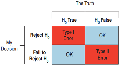
Type I Error

• Reject \(H_0\) when \(H_0\) is true.

Type II Error

• Fail to reject \(H_0\) when \(H_0\) is false.

Medicine: Such as an AIDS test

• Type I Error → False positive: Healthy person is diagnosed with the disease.
• Type II Error → False negative: Infected person is diagnosed as disease free.

Type I and II Errors

Which one is worse?

Jury Decisions

• Type I: Found guilty when the defendant is innocent. Put an innocent person in jail.
• Type II: Not enough evidence to convict, but was guilty. A murderer goes free.

Probabilities of Type I and II Errors

• P(Type I Error) = \(\alpha\)
  • This represents the probability that if \(H_0\) is true then we will reject \(H_0\).
• P(Type II Error) = \(\beta\)
  • We cannot calculate \(\beta\). Saying \(H_0\) is false does not tell us what the parameter is.
• Decreasing \(\alpha\) results in an increase of \(\beta\).
• The only way to decrease both is to increase the sample size.

Diabetes Drug Revisited

The study found patients who took the drug had an increased risk of heart attack.

• What kind of error if their findings were due to chance?
  • \(H_0\) is true but they rejected \(H_0\).
  • Type I error.
  • Patients would be deprived of the diabetes drug’s benefits, when there is no increased risk of heart attack.

Power

The power of a test is the probability it will correctly reject \(H_0\) when \(H_0\) is false.

• Power = 1 – \(\beta\)
• If a study fails to reject \(H_0\), either
  • \(H_0\) was true. No error was made.
  • \(H_0\) is false. Type II error was made.

Diabetes Drug Study

The meta study resulted in a new larger study of 47 different trials.

• How could this larger sample size help?
  • Increasing the sample size increases the power of the analysis, increasing the chance of detecting the danger if there is one.

Effect Size

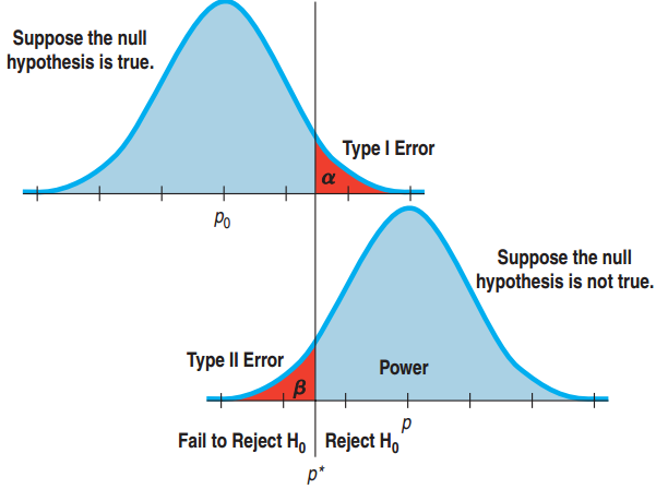
The distance between the null hypothesis (\(p_0\) for example) and the truth, p, is the effect size.

We don’t know the “true” p, so we estimate the effect size as difference between the null and the observed value.

• A small effect size is difficult to detect (high probability of Type II error)
• Power depends on effect size and standard deviation.
• “How big a difference would matter?”.
  • In detecting the “human energy field” would a 53% or a 75% success rate be remarkable?

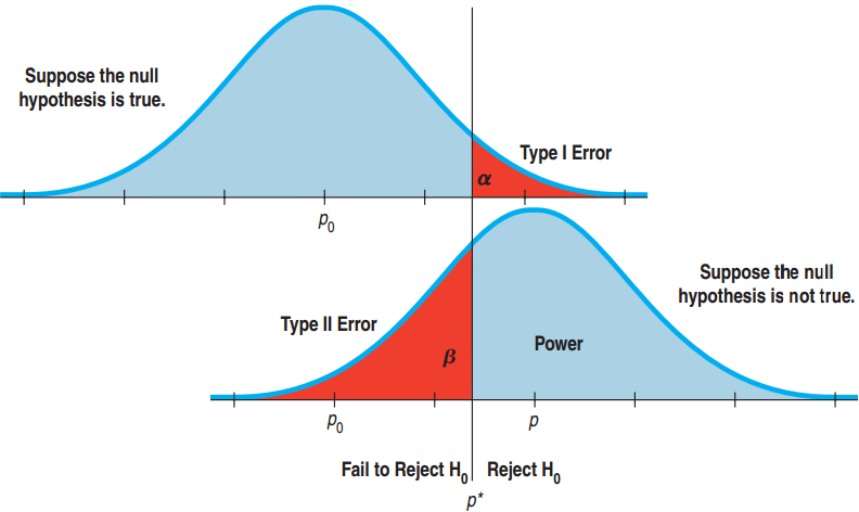
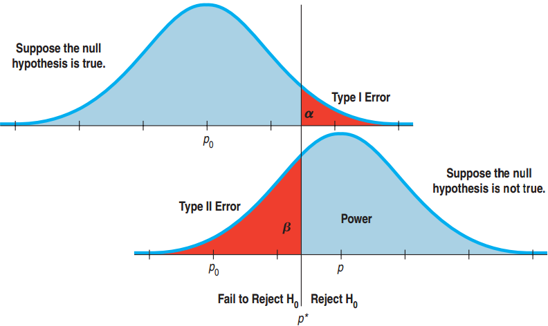
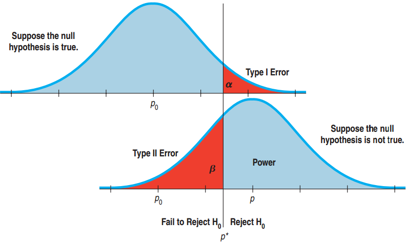
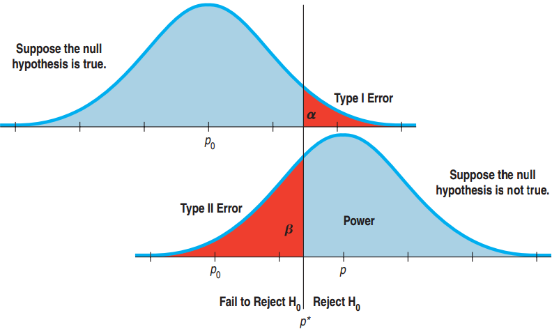
The Picture Explains It All

What We Get from the Picture

• Power = 1 – \(\beta\)
• Reducing \(\alpha\) to lower P(Type I) moves the critical value p* to the right. This increases \(\beta\), P(Type II), and decreases the power.
• The larger difference between p and \(p_0\), the smaller the chance of Type II error and greater the power.

Reducing Both Type I and II Errors?

• Reducing P(Type I Error) increases P(Type II Error).
• Reducing P(Type II Error) increases P(Type I Error).

• How can we reduce both?

Reducing both? Increase the sample size!

How can we reduce both?

• Increase the sample size!
  • SD goes down.
  • p* moves closer to \(p_0\).
  • \(\beta\) goes down.

Benefits of a Large Sample Size

The diabetes drug manufacturer looked at the study and rebutted that the sample size was too small.

• Why would this smaller study have been less likely to detect a difference in risks?
  • Small studies have more sampling variability.
  • Small studies have less power.
  • Large studies are better but very expensive.

What Can Go Wrong?

Don’t interpret the P-value as the probability that \(H_0\) is true.

• P-Value is about data, not the hypothesis.
• It is the probability of observing data this unusual given that \(H_0\) is true.

Don’t believe too strongly in arbitrary \(\alpha\) levels.

• P-value = 0.0499 and P-value = 0.0501 are basically the same.
• Often it is better to report just the P-value.

What Can Go Wrong?

Don’t confuse practical and statistical significance.

• A large sample size makes it easy to discern a trivial change from \(H_0\).
• A small sample size can make practically significant data statistically insignificant.

Don’t forget that in spite of all your care, you might make a wrong decision.

• We can’t reduce P(Type I) and P(Type II) to 0.

“Statistics means never having to say you’re certain.”