Quantitative Methods

Lecture 14

Serena DeStefani

2020-07-30

Quantitative Methods

Serena DeStefani – Lecture 14 – 7/30/2020

Announcements

• Let me know if you want to see the midterm
• Please return it back to me
• HW6 due today
• Datacamp due Monday

How to Define “Rare Enough”: threshold \(\alpha\)

• Need to make a decision whether P-value is low enough to reject H₀ → the value is too extreme to be likely to belong to the sampling distribution
• → Set a threshold value
• This is called the alpha level (\(\alpha\)).

• P-value < \(\alpha\):
  • Reject H₀.
  • The results are statistically significant.
• P-value > \(\alpha\):
  • Fail to reject H₀.
  • The results are not statistically significant.

21.5

Errors

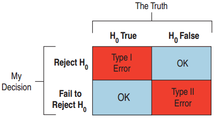
Type I and II Errors

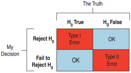
Type I Error

• Reject H₀ when H₀ is true.

Type II Error

• Fail to reject H₀ when H₀ is false.

Medicine: Such as an AIDS test

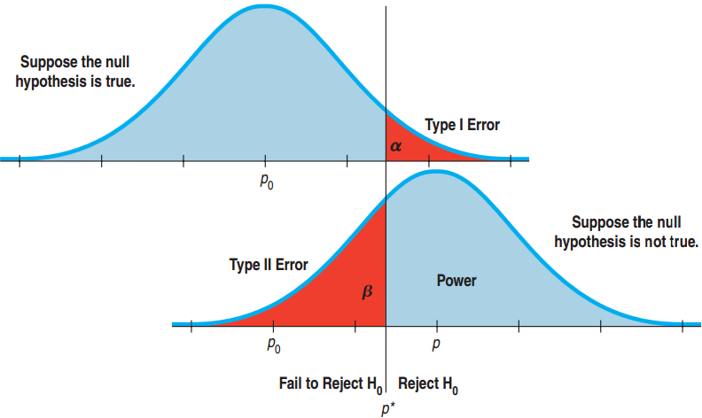
• Type I Error → False positive: Healthy person is diagnosed with the disease.
• Type II Error → False negative: Infected person is diagnosed as disease free.

Type I and II Errors

Jury Decisions

• Type I: Found guilty when the defendant is innocent. Put an innocent person in jail.
• Type II: Not enough evidence to convict, but was guilty. A murderer goes free.

Probabilities of Type I and II Errors

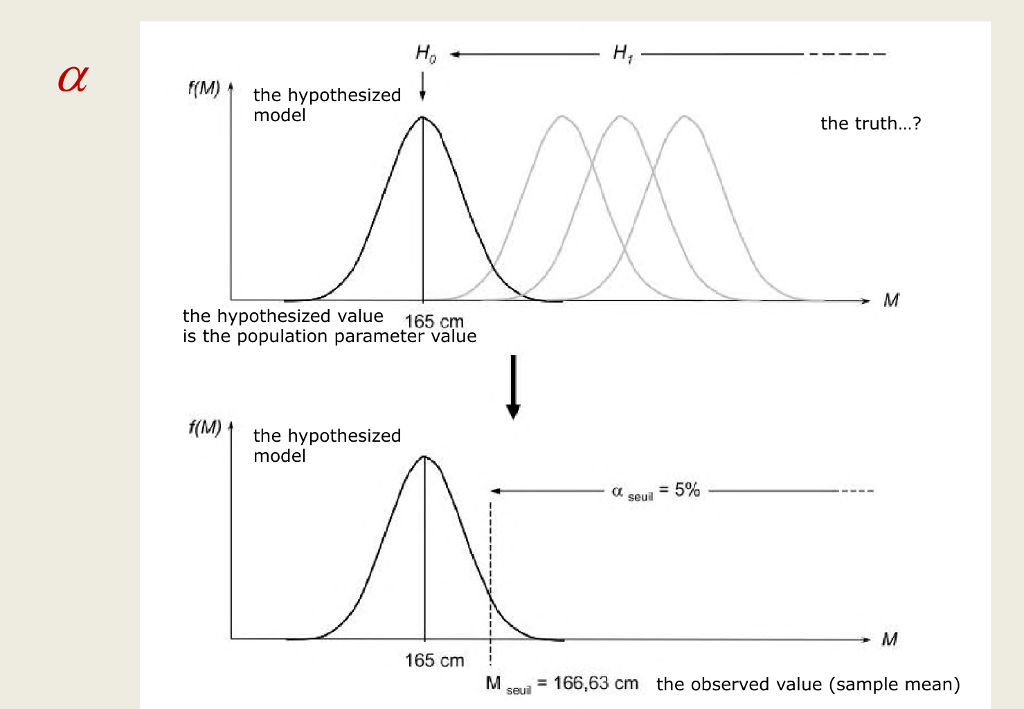
• P(Type I Error) = \(\alpha\)
  • This represents the probability that if H₀ is true then we will reject H₀.
• P(Type II Error) = \(\beta\)
  • We cannot calculate \(\beta\). Saying H₀ is false does not tell us what the parameter is.
• Decreasing \(\alpha\) results in an increase of \(\beta\).
• The only way to decrease both is to increase the sample size.

Diabetes Drug Revisited

The study found patients who took the drug had an increased risk of heart attack.

• What kind of error if their findings were due to chance?

• H₀ is true but they rejected H₀.
• Type I error.
• Patients would be deprived of the diabetes drug’s benefits, when there is no increased risk of heart attack.

Power

The power of a test is the probability it will correctly reject H₀ when H₀ is false.

• Power = \(1 - \beta\)

• If a study fails to reject H₀, either
  • H₀ was true. No error was made.
  • H₀ is false. Type II error was made.

Effect Size

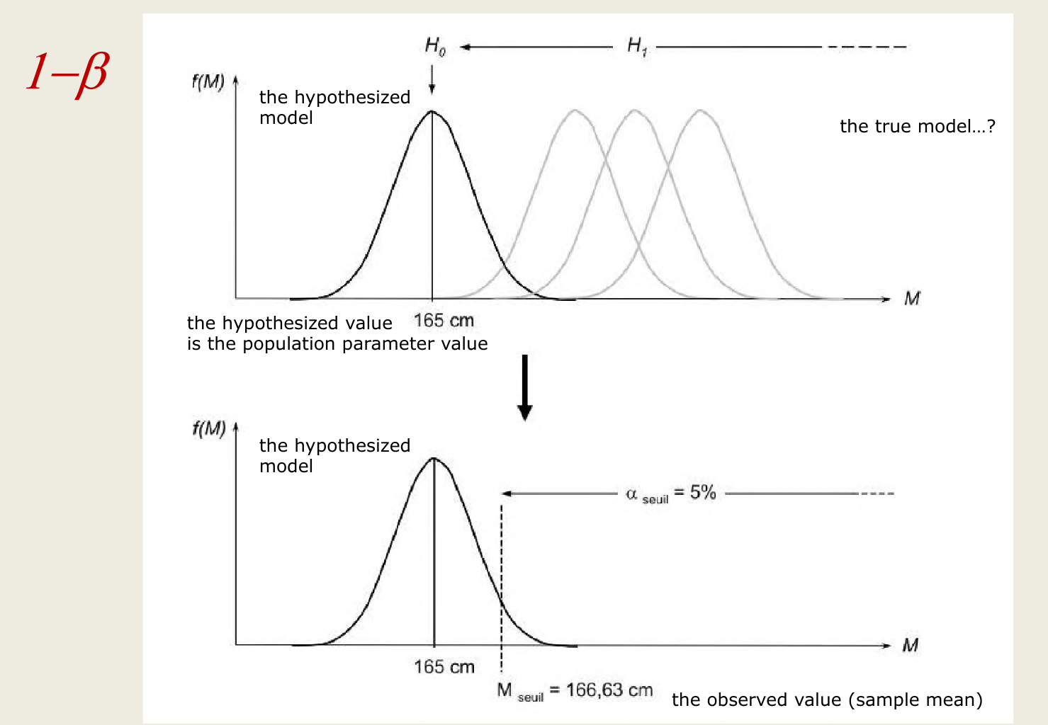
The distance between the null hypothesis (p₀, the population parameter, for example) and the truth, p (the true model population parameter), is the effect size.

We don’t know the true p, so we estimate the effect size as difference between the null and the observed value.

• A small effect size is difficult to detect (high probability of Type II error)
• Power depends on effect size and standard deviation.
• “How big a difference would matter?”.
  • In detecting the “human energy field” would a 53% or a 75% success rate be remarkable?

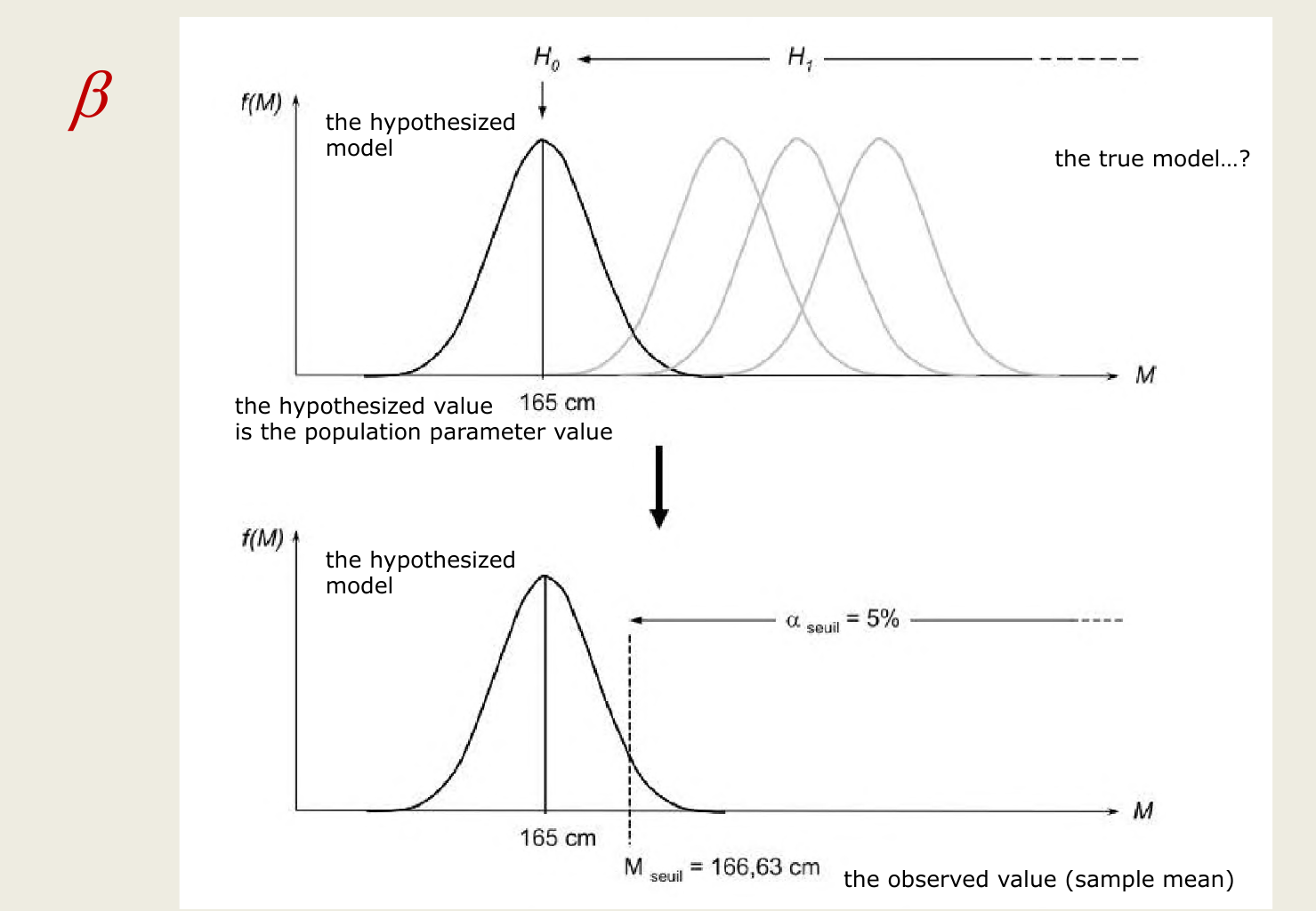
The Picture Explains It All

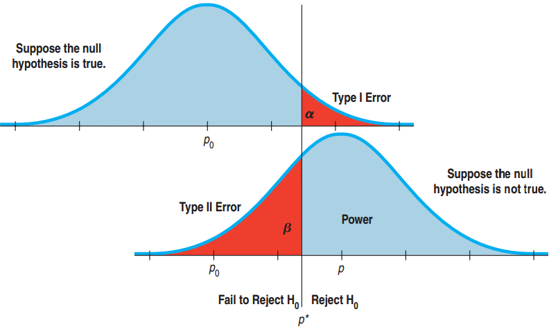
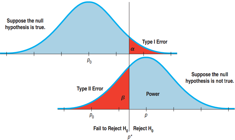
• In the top figure, if \(p_0\) is the true proportion, high \(\hat{p}\) results in a Type I error.
• In the bottom figure, if \(p\) is the true proportion, a low \(\hat{p}\) (near \(p_0\)) results in a Type II error.

What We Get from the Picture

• Power = \(1 - \beta\)
• Reducing \(\alpha\) to lower P(Type I) moves the critical value \(p^*\) to the right. This increases \(\beta\), P(Type II), and decreases the power.
• The larger difference between \(p\) and \(p_0\), the smaller the chance of Type II error and greater the power.

Reducing Both Type I and II Errors ?

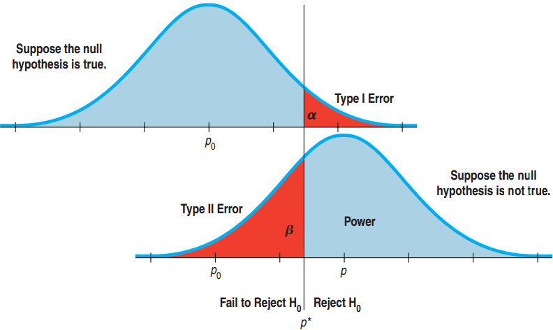
• Reducing P(Type I Error) increases P(Type II Error).
• Reducing P(Type II Error) increases P(Type I Error).

• How can we reduce both?

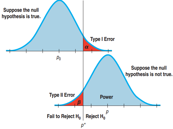
Reducing both? Increase the sample size!

• How can we reduce both?
• Increase the sample size!
  • SD goes down.
  • \(p^*\) moves closer to \(p_0\).
  • \(\beta\) goes down.

Benefits of a Large Sample Size

The diabetes drug manufacturer looked at the study and rebutted that the sample size was too small.

• Why would this smaller study have been less likely to detect a difference in risks?

• Small studies have more sampling variability.
• Small studies have less power.
• Large studies are better but very expensive.

What Can Go Wrong?

Don’t interpret the P-value as the probability that H₀ is true.

• P-Value is about data, not the hypothesis.
• It is the probability of observing data this unusual given that H₀ is true.

Don’t believe too strongly in arbitrary \(\alpha\) levels.

• P-value = 0.0499 and P-value = 0.0501 are basically the same.
• Often it is better to report just the P-value.

What Can Go Wrong?

Don’t confuse practical and statistical significance.

• A large sample size makes it easy to discern a trivial change from H₀.
• A small sample size can make practically significant data statistically insignificant.

Don’t forget that in spite of all your care, you might make a wrong decision.

• We can’t reduce P(Type I) and P(Type II) to 0.

“Statistics means never having to say you’re certain.”

Chapter 22

Comparing groups

22.1

The Standard Deviation of a Difference

Variance of the Differences Revisited

For independent variables X and Y

\[\text{Var}(X - Y) = \text{Var}(X) + \text{Var}(Y)\]

• The variance of the difference is larger than either.
  • Many 16-ounce cereal boxes vary from box to box. If everyone pours about 2 ounces from their box, then the variance of the difference between the original and the poured amount will be more than the variance had each box been exactly 16 ounces.
• Take a square root to get

\[SD(X - Y) = \sqrt{SD(X)^2 + SD(Y)^2}\]

The Standard Deviation of the Difference Between Two Proportions

• Use subscripts to show two proportions:

\[p_1,\ q_1,\ p_2,\ q_2,\ \hat{p}_1,\ \hat{p}_2,\ n_1,\ n_2\]

The Standard Deviation of the Difference Between Two Proportions

• Use subscripts to show two proportions:

\[p_1,\ q_1,\ p_2,\ q_2,\ \hat{p}_1,\ \hat{p}_2,\ n_1,\ n_2\]

• Var(X – Y) = Var(X) + Var(Y)

\[\text{Var}(\hat{p}_1 - \hat{p}_2) =\]

The Standard Deviation of the Difference Between Two Proportions

• Use subscripts to show two proportions:

\[p_1,\ q_1,\ p_2,\ q_2,\ \hat{p}_1,\ \hat{p}_2,\ n_1,\ n_2\]

• Var(X – Y) = Var(X) + Var(Y)

\[\text{Var}(\hat{p}_1 - \hat{p}_2) = \left(\sqrt{\frac{p_1 q_1}{n_1}}\right)^2 + \left(\sqrt{\frac{p_2 q_2}{n_2}}\right)^2 = \frac{p_1 q_1}{n_1} + \frac{p_2 q_2}{n_2}\]

The Standard Deviation of the Difference Between Two Proportions

• Use subscripts to show two proportions:

\[p_1,\ q_1,\ p_2,\ q_2,\ \hat{p}_1,\ \hat{p}_2,\ n_1,\ n_2\]

\[\text{Var}(\hat{p}_1 - \hat{p}_2) = \left(\sqrt{\frac{p_1 q_1}{n_1}}\right)^2 + \left(\sqrt{\frac{p_2 q_2}{n_2}}\right)^2 = \frac{p_1 q_1}{n_1} + \frac{p_2 q_2}{n_2}\]

\[SD(\hat{p}_1 - \hat{p}_2) =\]

The Standard Deviation of the Difference Between Two Proportions

• Use subscripts to show two proportions:

\[p_1,\ q_1,\ p_2,\ q_2,\ \hat{p}_1,\ \hat{p}_2,\ n_1,\ n_2\]

\[\text{Var}(\hat{p}_1 - \hat{p}_2) = \left(\sqrt{\frac{p_1 q_1}{n_1}}\right)^2 + \left(\sqrt{\frac{p_2 q_2}{n_2}}\right)^2 = \frac{p_1 q_1}{n_1} + \frac{p_2 q_2}{n_2}\]

\[SD(\hat{p}_1 - \hat{p}_2) = \sqrt{\frac{p_1 q_1}{n_1} + \frac{p_2 q_2}{n_2}}\]

• Standard Error:

The Standard Deviation of the Difference Between Two Proportions

• Use subscripts to show two proportions:

\[p_1,\ q_1,\ p_2,\ q_2,\ \hat{p}_1,\ \hat{p}_2,\ n_1,\ n_2\]

\[\text{Var}(\hat{p}_1 - \hat{p}_2) = \left(\sqrt{\frac{p_1 q_1}{n_1}}\right)^2 + \left(\sqrt{\frac{p_2 q_2}{n_2}}\right)^2 = \frac{p_1 q_1}{n_1} + \frac{p_2 q_2}{n_2}\]

• Standard Deviation

\[SD(\hat{p}_1 - \hat{p}_2) = \sqrt{\frac{p_1 q_1}{n_1} + \frac{p_2 q_2}{n_2}}\]

• Standard Error (use for CI):

\[SE(\hat{p}_1 - \hat{p}_2) = \sqrt{\frac{\hat{p}_1 \hat{q}_1}{n_1} + \frac{\hat{p}_2 \hat{q}_2}{n_2}}\]

Standard Deviation of a Difference

57% of 248 boys aged 15-17 have online profiles. 70% of 256 girls aged 15-17 have online profiles.

• What is the standard error of the difference?
  • The boys and girls were selected at random, so independent

\[SE(\hat{p}_{boys}) = \sqrt{\frac{(0.57)(0.43)}{248}} \approx 0.0314 \qquad SE(\hat{p}_{girls}) = \sqrt{\frac{(0.70)(0.30)}{256}} \approx 0.0286\]

\[SE(\hat{p}_{boys} - \hat{p}_{girls}) = \sqrt{0.0314^2 + 0.0286^2} \approx 0.0425\]

\[SD(X - Y) = \sqrt{SD(X)^2 + SD(Y)^2}\]

22.2

Assumptions and Conditions for Comparing Proportions

Independence

Independence Assumption: Check

• Randomization Condition: The data are drawn independently and randomly.
• 10% Condition: If data sampled without replacement, the data represent less than 10% of the population.

Independent Groups Assumption

• The two groups are independent of each other.
  • Comparing wives and husbands or before and after can give a smaller difference between SDs.

Sample size

• Successes and Failures for both ≥ 10

22.3

A Confidence Interval for the Difference Between Two Proportions

Review: Sampling Distribution for One Proportion

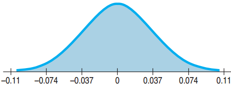
Sampling Distribution for the Difference Between Two Independent Proportions

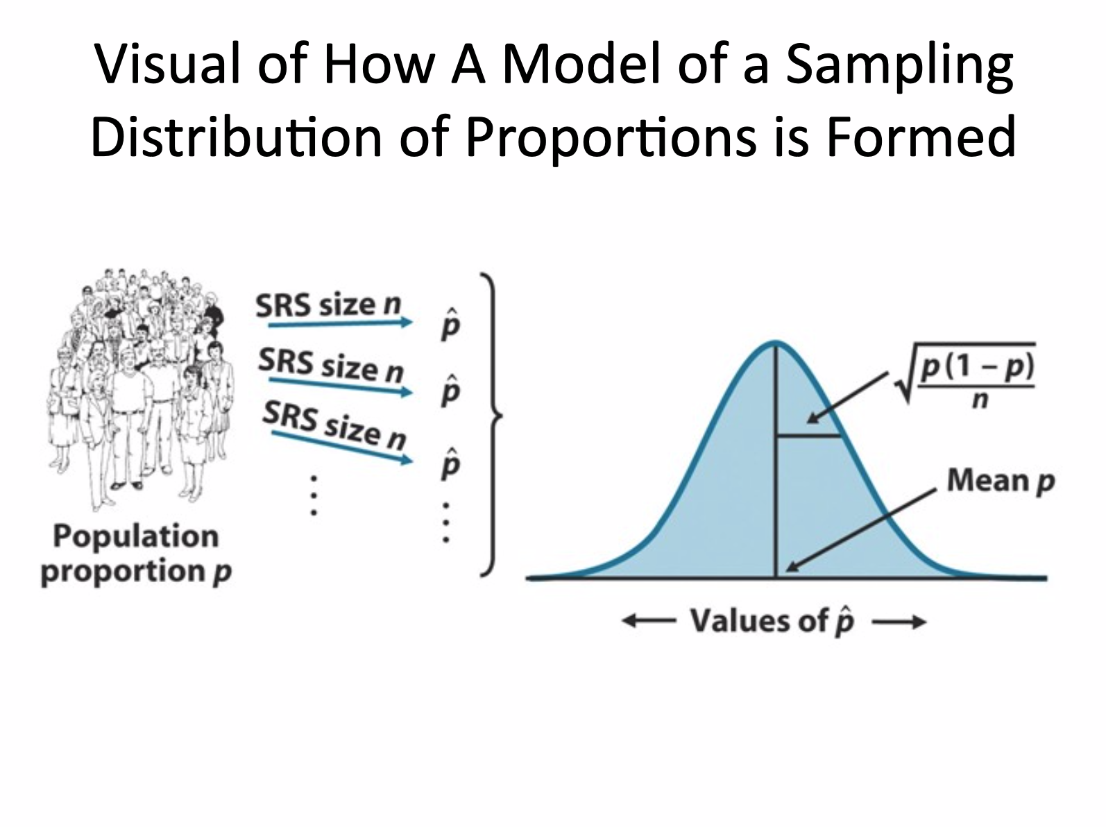
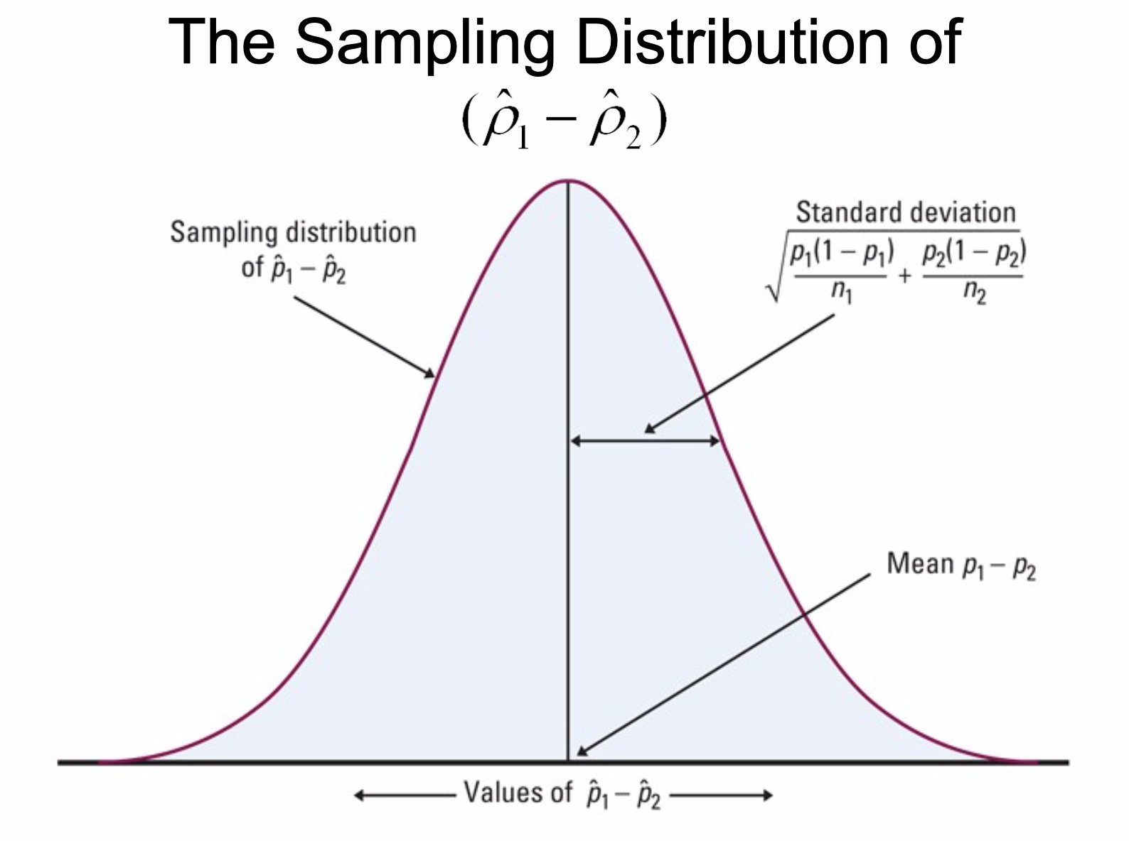
If samples are independent (individually and by groups) and the sample sizes are large, then the sampling distribution of \(\hat{p}_1 - \hat{p}_2\)

• Follows a Normal model
• Has mean \(\mu = p_1 - p_2\)
• Has standard deviation (use population proportion!)

\[SD(\hat{p}_1 - \hat{p}_2) = \sqrt{\frac{p_1 q_1}{n_1} + \frac{p_2 q_2}{n_2}}\]

Two-Proportion z-Interval

If the conditions are met, the confidence interval for \(p_1 - p_2\) is (use SE calculated with sample proportions!)

\[(\hat{p}_1 - \hat{p}_2) \pm z^* \times SE(\hat{p}_1 - \hat{p}_2)\]

\[SE(\hat{p}_1 - \hat{p}_2) = \sqrt{\frac{\hat{p}_1 \hat{q}_1}{n_1} + \frac{\hat{p}_2 \hat{q}_2}{n_2}}\]

• \(z^*\) is the critical value that corresponds to the confidence level C – you can get it from the z table

Online Presence: Boys vs. Girls

• 57% of the 248 boys had online profiles.
• 70% of the 256 girls had online profiles.
• What does the confidence interval say about the difference?

Online Presence: Boys vs. Girls

• 57% of the 248 boys had online profiles.
• 70% of the 256 girls had online profiles.
• What does the confidence interval say about the difference?

\[(\hat{p}_{girls} - \hat{p}_{boys}) \pm z^* \times SE(\hat{p}_{girls} - \hat{p}_{boys})\]

\[(0.7 - 0.57) \pm 1.96 \times 0.0425\]

\[(4.7\%,\ 21.3\%)\]

• We are 95% confident that the proportion of teen girls who post online is between 4.7% and 21.3% higher than for boys.

Wearing Seat Belts

Question: How much difference is there in the proportion of male drivers who wear seat belts when sitting next to a man and the proportion when sitting next to a woman?

• Plan: Want a 95% confidence interval for \(p_F - p_M\).
• Data are from a random sample of MA drivers.

Wearing Seat Belts

Model:

• Randomization Condition: Participants selected randomly and independently from car to car.
• 10% Condition: Sample size is less than 10% of all drivers.
• Independent Groups Assumption: The seat-belt use with male and female passengers are independent.

Wearing Seat Belts

Model:

• Success Failure Condition:
  • With female passengers: 2777 wore seat belts, 1431 did not.
  • With male passengers: 1363 wore seat belts, 1400 did not.
  • All successes and failures ≥ 10.
• All conditions are met. Use the Normal model and find a 2-proportion z-interval.

Wearing Seat Belts

• Mechanics: \(n_F\) = 4208, \(n_M\) = 2763
  • With female passengers: 2777 wore seat belts
  • With male passengers: 1363 wore seat belts

Wearing Seat Belts

• Mechanics: \(n_F\) = 4208, \(n_M\) = 2763

\[\hat{p}_F = \frac{2777}{4208} \approx 0.660, \quad \hat{p}_M = \frac{1363}{2763} \approx 0.493\]

\[SE(\hat{p}_F - \hat{p}_M) = \sqrt{\frac{\hat{p}_F \hat{q}_F}{n_F} + \frac{\hat{p}_M \hat{q}_M}{n_M}} = \sqrt{\frac{(0.660)(0.340)}{4208} + \frac{(0.493)(0.507)}{2763}} \approx 0.012\]

\[ME = z^* \times SE(\hat{p}_F - \hat{p}_M) \approx 1.96 \times 0.012 \approx 0.024\]

\[\hat{p}_F - \hat{p}_M = 0.660 - 0.493 = 0.167\]

\[95\%\ \text{CI}: 0.167 \pm 0.024 = (14.3\%,\ 19.1\%)\]

Wearing Seat Belts

• Conclusion: I am 95% confident that the proportion of male drivers who wear seat belts when driving next to a female passenger is between 14.3 and 19.1 percentage points higher than the proportion who wear seat belts when driving next to a male passenger.

Caution

• Can’t generalize to other states
• Can’t say men buckle up because of the women; Lurking variables such as age may be present.

22.4

The Two Sample z-Test: Testing for the Difference Between Proportions

Internet Before Sleep

The Sleep in America Poll found that 205 of 293, or 70%, of Gen-Y use the Internet before sleep. 235 of 469, or 50%, of Gen-X use the Internet before sleep.

• Is this difference of 20% real or is it likely to be due only to natural fluctuations in the sample?
• What’s the null hypothesis?

Internet Before Sleep

The Sleep in America Poll found that 205 of 293, or 70%, of Gen-Y use the Internet before sleep. 235 of 469, or 50%, of Gen-X use the Internet before sleep.

• Is this difference of 20% real or is it likely to be due only to natural fluctuations in the sample?
  • H₀: \(p_1 - p_2 = 0\)
• For CI:

\[SE(\hat{p}_1 - \hat{p}_2) = \sqrt{\frac{\hat{p}_1 \hat{q}_1}{n_1} + \frac{\hat{p}_2 \hat{q}_2}{n_2}}\]

• For hypothesis testing, we can do slightly better.

Pooling the Proportion

• H₀ says the proportions are equal.
• To do a hypothesis test, we assume that the proportions are equal
• We should have only one value for proportion
• Total successes: 205 + 235 = 440
• Total trials: 293 + 469 = 762
• Pooled Proportion:

\[\hat{p}_{pooled} = \frac{Success_1 + Success_2}{n_1 + n_2} = \frac{440}{762} \approx 0.5774\]

Standard Error for Internet Before Sleep

The Sleep in America Poll found that 205 of 293 or 70% of Gen-Y use the Internet before sleep. 235 of 469 or 50% of Gen-X use the Internet before sleep.

Standard Error for Internet Before Sleep

The Sleep in America Poll found that 205 of 293 or 70% of Gen-Y use the Internet before sleep. 235 of 469 or 50% of Gen-X use the Internet before sleep.

\[SE_{pooled}(\hat{p}_1 - \hat{p}_2) = \sqrt{\frac{\hat{p}_{pooled}\,\hat{q}_{pooled}}{n_1} + \frac{\hat{p}_{pooled}\,\hat{q}_{pooled}}{n_2}}\]

\[= \sqrt{\frac{0.5774(1 - 0.5774)}{293} + \frac{0.5774(1 - 0.5774)}{469}} \approx 0.0368\]

Two-Proportion z-Test

• Conditions same as 2-proportion CI.
• H₀: \(p_1 - p_2 = 0\)

\[\hat{p}_{pooled} = \frac{Success_1 + Success_2}{n_1 + n_2}\]

\[SE_{pooled}(\hat{p}_1 - \hat{p}_2) = \sqrt{\frac{\hat{p}_{pooled}\,\hat{q}_{pooled}}{n_1} + \frac{\hat{p}_{pooled}\,\hat{q}_{pooled}}{n_2}}\]

\[z = \frac{\hat{p}_1 - \hat{p}_2 - 0}{SE_{pooled}(\hat{p}_1 - \hat{p}_2)}\]

• The statistic follows the Normal model.

Pre-Sleep Internet Rates Differ?

• Plan: Random sample of adults: 293 Gen Y (205), 469 Gen X (235)
• Hypotheses:
  • H₀: \(p_{GenY} - p_{GenX} = 0\)
  • H_A: \(p_{GenY} - p_{GenX} \neq 0\)
• Model
  • Randomization Condition: Randomly selected and stratified by sex.

Pre-Sleep Internet Rates Differ?

• Model (Continued)
  • 10% Condition: Samples less than 10% of all Gen X and Gen Y.
  • Independent Groups Assumption: The samples were selected at random so independent.
  • Success/Failure Condition: Observed numbers of successes and failures for both groups ≥ 10.
• The conditions are all met. Use the Normal model and perform a two-proportion z-test.

Pre-Sleep Internet Rates Differ?

• Mechanics:

\[n_{GenY} = 293,\ y_{GenY} = 205,\ \hat{p}_{GenY} = 0.700\]

\[n_{GenX} = 469,\ y_{GenX} = 235,\ \hat{p}_{GenX} = 0.501\]

Pre-Sleep Internet Rates Differ?

• Mechanics:

\[n_{GenY} = 293,\ y_{GenY} = 205,\ \hat{p}_{GenY} = 0.700\]

\[n_{GenX} = 469,\ y_{GenX} = 235,\ \hat{p}_{GenX} = 0.501\]

\[\hat{p}_{pooled} = \frac{y_{GenY} + y_{GenX}}{n_{GenY} + n_{GenX}} = \frac{205 + 235}{293 + 469} \approx 0.5774\]

\[SE_{pooled}(\hat{p}_{GenY} - \hat{p}_{GenX}) = \sqrt{\frac{\hat{p}_{pooled}(1 - \hat{p}_{pooled})}{n_{GenY}} + \frac{\hat{p}_{pooled}(1 - \hat{p}_{pooled})}{n_{GenX}}}\]

\[= \sqrt{\frac{(0.5774)(0.4226)}{293} + \frac{(0.5774)(0.4226)}{469}} \approx 0.0368\]

Pre-Sleep Internet Rates Differ?

• Mechanics: (Continued)

\[\hat{p}_{GenY} - \hat{p}_{GenX} = 0.700 - 0.501 = 0.199\]

\[z = \frac{(\hat{p}_{GenY} - \hat{p}_{GenX}) - 0}{SE_{pooled}(\hat{p}_{GenY} - \hat{p}_{GenX})}\]

\[= \frac{0.199}{0.0368} \approx 5.41\]

• P-value = 2 × P(z > 5.41) ≤ 0.0001

Pre-Sleep Internet Rates Differ?

• Conclusion:
  • P-value ≤ 0.0001: If there really was no difference in surfing rates between the two groups, then the difference observed in this study would be very rare indeed.
  • We can conclude that there is, in fact, a difference in the rate of surfing between GenY and GenX adults.

Easy to Find Teens Online: Girls vs. Boys

19% (62 girls) of 325 girls and 28% (75 boys) of 268 boys have easy to find online profiles.

• Is there a real difference between all boys and girls?
  • H₀: \(p_{boys} - p_{girls} = 0\)
  • H_A: \(p_{boys} - p_{girls} \neq 0\)
• Randomization Condition: Both samples randomly and independently chosen
• 10% Condition: Sample sizes certainly less than 10% of all boys and girls

Easy to Find Teens Online: Girls vs. Boys

• Independent Groups Assumption: The boys are independent of the girls.
• Success/Failure Condition:
  • Girls: 62 successes and 263 failures.
  • Boys: 75 successes and 193 failures.
• Use the two-proportion z-test.

Easy to Find Teens Online: Girls vs. Boys

\[\hat{p}_{pooled} = \frac{75 + 62}{268 + 325} \approx 0.231\]

\[SE_{pooled}(\hat{p}_{boys} - \hat{p}_{girls}) = \sqrt{\frac{0.231 \times 0.769}{268} + \frac{0.231 \times 0.769}{325}} \approx 0.0348\]

\[z = \frac{(0.28 - 0.19) - 0}{0.0348} \approx 2.59 \qquad P(z > 2.59) \approx 0.0048\]

• Two-Tailed Test: P-value = 2(0.0048) = 0.0096
• P-value very small → Reject H₀
• There is strong evidence to say that there is a difference between the proportions of boys and girls who say they are easy to find online.

22.5

A Confidence Interval for the Difference Between Two Means

Difference Between Means: Standard Error

\[\text{Var}(\bar{y}_1 - \bar{y}_2) = \text{Var}(\bar{y}_1) + \text{Var}(\bar{y}_2)\]

\[SD(\bar{y}_1 - \bar{y}_2) = \sqrt{\text{Var}(\bar{y}_1) + \text{Var}(\bar{y}_2)}\]

\[SD(\bar{y}_1 - \bar{y}_2) = \sqrt{\frac{\sigma_1^2}{n_1} + \frac{\sigma_2^2}{n_2}}\]

• Don’t know the population \(\sigma\), so use the samples s:

\[SE(\bar{y}_1 - \bar{y}_2) = \sqrt{\frac{s_1^2}{n_1} + \frac{s_2^2}{n_2}}\]

Effect of Knowing How Much We Eat

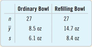
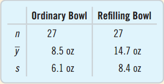
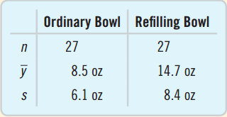
• 27 people observed eating soup from ordinary bowl.
• 27 people observed eating soup from a bowl that slowly refills without the person knowing.
• Find the standard error.

\[SE(\bar{y}_{refill} - \bar{y}_{ordinary}) = \sqrt{\frac{s_r^2}{n_r} + \frac{s_o^2}{n_o}} = \sqrt{\frac{8.4^2}{27} + \frac{6.1^2}{27}} \approx 2.0 \text{ oz.}\]

Sampling Distribution for the Difference Between Two Means

• When the assumptions are met, the sampling distribution for the difference between two independent means:

\[t = \frac{(\bar{y}_1 - \bar{y}_2) - (\mu_1 - \mu_2)}{SE(\bar{y}_1 - \bar{y}_2)} \qquad SE(\bar{y}_1 - \bar{y}_2) = \sqrt{\frac{s_1^2}{n_1} + \frac{s_2^2}{n_2}}\]

• Uses the Student’s t-model
• The degrees of freedom are complicated, so just use a computer.

Assumptions and Conditions

Independence

• Same assumptions as proportions
• Between and within groups
• Randomization is evidence of independence.
• If not independent, can you use pairing?

Nearly Normal Condition

• Same as with a single mean, but must check both.
• n < 15: must be very close to normal.
• 15 ≤ n ≤ 40: Check for outliers and skewness.
• n > 40: Fine as long as no extreme outliers or extreme skewness

Checking Conditions for Soup Experiment

• Randomization Condition: The subjects were randomly assigned.
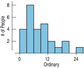
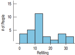
• Nearly Normal Condition: n = 27 for both. Histograms only a little skewed. No outliers.
• Independent Groups Assumption: Randomization to treatment groups guarantees this
• Okay to construct a two-sample t-interval for the difference between two means.

Two-Sample t-Interval for the Difference Between Two Means

• When the conditions are met, the confidence interval for the difference between means from two independent groups is

\[(\bar{y}_1 - \bar{y}_2) \pm t^*_{df} \times SE(\bar{y}_1 - \bar{y}_2)\]

\[SE(\bar{y}_1 - \bar{y}_2) = \sqrt{\frac{s_1^2}{n_1} + \frac{s_2^2}{n_2}}\]

Confidence Interval for Soup Experiment

• What does a 95% confidence interval say about the difference in mean amounts eaten?

\[t^*_{df} = 2.011 \text{ (by computer)}\]

Confidence Interval for Soup Experiment

• What does a 95% confidence interval say about the difference in mean amounts eaten?

\[\bar{y}_{refill} - \bar{y}_{ordinary} = 14.7 - 8.5 = 6.2\]

\[t^*_{df} = 2.011 \text{ (by computer)}\]

\[ME = t^*_{df} \times SE(\bar{y}_{refill} - \bar{y}_{ordinary}) = 2.011 \times 2.0 \approx 4.02\]

\[\text{CI}: 6.2 \pm 4.02 = (2.18,\ 10.22)\]

• I am 95% confident that people eating from a refilling bowl will eat between 2.18 and 10.22 more ounces than those eating from an ordinary bowl.

22.6

The Two-Sample t-Test: Testing for the Difference Between Two Means

Two-Sample t-Test for the Difference Between Means

• Conditions same as two-sample t-interval
• H₀: \(\mu_1 - \mu_2 = \Delta_0\) (\(\Delta_0\) usually 0)

\[t = \frac{(\bar{y}_1 - \bar{y}_2) - \Delta_0}{SE(\bar{y}_1 - \bar{y}_2)} \qquad SE(\bar{y}_1 - \bar{y}_2) = \sqrt{\frac{s_1^2}{n_1} + \frac{s_2^2}{n_2}}\]

• When the conditions are met and the null hypothesis is true, use the Student’s t-model to find the P-value.

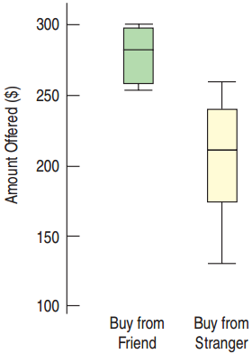
Do People Offer a Lower Price to Friends than to Strangers?

Is there a difference in the average price for a used camera people would offer a friend and a stranger?

• Plan: I have bid prices from 8 subjects buying from a friend and 7 buying from a stranger, found in a randomized experiment.
• Hypotheses
  • H₀: \(\mu_F - \mu_S = 0\)
  • H_A: \(\mu_F - \mu_S \neq 0\)

Friends vs. Strangers

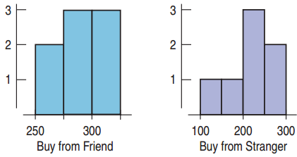
• Model: Has practical significance, but is there statistical significance?
  • Randomization Condition: Subjects assigned to treatment groups randomly.
  • Independent Groups Assumption: Randomizing gives independent groups.

Friends vs. Strangers

• Model (Continued):
  • Nearly Normal Condition: Histograms are reasonably unimodal and symmetric, but with the very small sample sizes, we should be concerned.
• The assumptions and conditions are somewhat reasonable.
• Use the Student’s t-model to perform a two-sample t-test.

Friends vs. Strangers

• Mechanics:

\[n_F = 8,\ n_S = 7\]

\[\bar{y}_F = \$281.88,\ \bar{y}_S = \$211.43\]

\[s_F = \$18.31,\ s_S = \$46.43\]

Friends vs. Strangers

• Mechanics:

\[n_F = 8,\ n_S = 7\]

\[\bar{y}_F = \$281.88,\ \bar{y}_S = \$211.43\]

\[s_F = \$18.31,\ s_S = \$46.43\]

\[SE(\bar{y}_F - \bar{y}_S) = \sqrt{\frac{18.31^2}{8} + \frac{46.43^2}{7}} \approx 18.70\]

\[\bar{y}_F - \bar{y}_S = 281.88 - 211.43 = \$70.45\]

\[t = \frac{70.45}{18.70} \approx 3.77\]

\[\text{P-value} = 2 \times P(t > 3.77) = 0.006\]

Friends vs. Strangers

• Conclusion: The P-value = 0.006 is very small.
• If there were no difference in the mean prices, then a difference this large would occur 6 times in 1000.
• Too rare to believe
• Reject H₀.
• Conclude that people are likely, on average, to offer a friend more than they’d offer a stranger for a used camera.

Difference in Donations Based on Images?

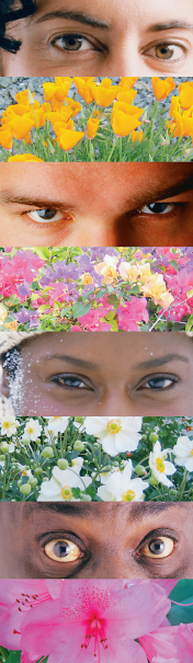
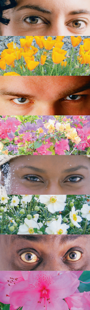
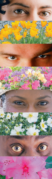
The cupboard next to the coffee station’s voluntary honesty box had alternating pictures of eyes and flowers each week.

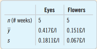
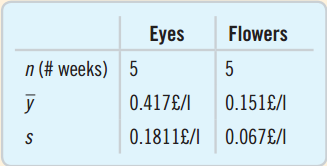
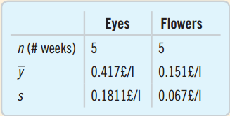
• Do these results provide evidence of a difference in mean donation when the eyes are shown and when the flowers are shown? Measured # pounds collected per liter of milk

Eyes vs. Flowers?

• H₀: \(\mu_{eyes} - \mu_{flowers} = 0\)
• H_A: \(\mu_{eyes} - \mu_{flowers} \neq 0\)

 

• Independence Assumption: The study is observational not randomized, but independence is probably true.
• Nearly Normal Condition: This should be checked.
• Independent Groups Assumption: Week-to-week independence is plausible.
• Do a two-sample t-test for the difference.

Eyes vs. Flowers

Eyes vs. Flowers

\[SE(\bar{y}_{eyes} - \bar{y}_{flowers}) = \sqrt{\frac{0.1811^2}{5} + \frac{0.067^2}{5}} \approx 0.0864\]

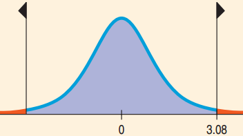
\[t = \frac{0.417 - 0.151}{0.0864} = 3.08\]

\[\text{P-value} = 2 \times P(t > 3.08) = 0.027\]

Eyes vs. Flowers?

• Assuming normal distributions, with P-value = 0.027, I will reject the null hypothesis.
• This study provides evidence that there is a difference in the mean amount of money people donate at the coffee station when there are flowers and when there are “eyes watching.”

22.7

The Pooled t-Test: Everyone Into the Pool?

Pooling

If the variances are equal, we can use pooling.

• Advantages of Pooling
  • Can have more degrees of freedom than two sample t-test.
  • More degrees of freedom gives a higher power.
• Disadvantage of Pooling
  • The assumption of equal variances is difficult to establish and often false.

Pooled Variance and Standard Error

• Pooled Variance:

\[s^2_{pooled} = \frac{(n_1 - 1)s_1^2 + (n_2 - 1)s_2^2}{(n_1 - 1) + (n_2 - 1)}\]

• Pooled Standard Error:

\[SE_{pooled} = \sqrt{\frac{s^2_{pooled}}{n_1} + \frac{s^2_{pooled}}{n_2}} = s_{pooled}\sqrt{\frac{1}{n_1} + \frac{1}{n_2}}\]

Pooled t-Test and Confidence Interval for Means

• Conditions same as two-sample t-interval/test plus the variances must be equal.
• H₀: \(\mu_1 - \mu_2 = \Delta_0\) (\(\Delta_0\) usually 0)

\[t = \frac{(\bar{y}_1 - \bar{y}_2) - \Delta_0}{SE_{pooled}(\bar{y}_1 - \bar{y}_2)} \qquad SE(\bar{y}_1 - \bar{y}_2) = s_{pooled}\sqrt{\frac{1}{n_1} + \frac{1}{n_2}}\]

\[s^2_{pooled} = \frac{(n_1 - 1)s_1^2 + (n_2 - 1)s_2^2}{(n_1 - 1) + (n_2 - 1)}\]

Pooled t-Test and Confidence Interval for Means (Continued)

• When the conditions are met and the null hypothesis is true, use the Student’s t-model with \((n_1 - 1) + (n_2 - 1)\) degrees of freedom.
• Use the model to find the P-value or margin of error.
• The CI is \((\bar{y}_1 - \bar{y}_2) \pm t^*_{df} \times SE_{pooled}(\bar{y}_1 - \bar{y}_2)\).
• df = \((n_1 - 1) + (n_2 - 1)\)
• The \(t^*\) depends on the confidence level.

When to Use the Pooled t-Test

• The pooled t-test has almost no advantage over the independent sample t-test.
• A great disadvantage is that the pooled t-test is very poor when the standard deviations are not the same.
• Avoid this test unless you are very certain that the variances (standard deviations) are the same.

What Can Go Wrong?

Don’t use two-sample methods when the samples aren’t independent.

• Random sampling is best.
• Consider matched-pairs design for dependent data.

Look at the plots.

• Boxplots, histograms, and normal plots will help you determine if the Near Normal Condition is met.
• A strong outlier can completely change the conclusions.

What Can Go Wrong?

Be cautious if you apply inference methods where there was no randomization.

• Without randomization, the inferences about the differences may be wrong.

Don’t interpret a significant difference in proportions or means causally.

• People with higher incomes are more likely to snore.
• Will surgery to prevent snoring make you rich?
• Maybe the lurking variable, age, causes both.

Announcements

• Let me know if you want to see the midterm
• Please return it back to me
• HW6 due today
• Datacamp due Monday