Quantitative Methods
Lecture 15
2020-08-03
Review
Pairing
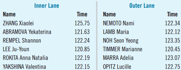
- Speed-skating races run in pairs. One starts in the inner lane, the other in the outer lane.
- Above are some of the randomly assigned pairs.
- The data are paired rather than independent.
- Blocking involves pairing arising from an experiment.
- Matching involves pairing arising from an observational study.
- With pairing, we look at the differences.
Comparing Mileage
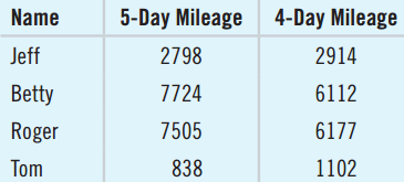
Do flexible schedules reduce total mileage? The table shows some workers’ mileage before and after the company switched to a 4-day work week.
- Why are these data paired?
- Each driver’s mileage recorded before and after.
- Not independent since we expect a high “before” mileage to predict a high “after” mileage.
- Paired because the differences such as Jeff: 2798 – 2914 = –116 have meaning.
Differences for Speed-Skater Pairs
- For paired data, create a new data set of the differences.
- We can now look only at the differences.
- Ignoring the original data, we now have a single data set.
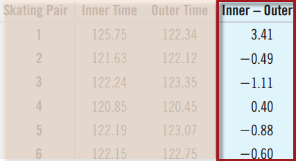
- Proceed with a one-sample t-test. This process is called a paired t-test.
4-Day vs. 5-Day Mileage
Is it okay to use these data to test whether the new schedule changed the amount of driving?
- Paired Data Condition: Before and after study
- Independence Assumption: The driving behavior of one worker is independent of another.
- Randomization Condition: The work trips randomly occurred.
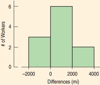
- Nearly Normal Condition: The sample size is small, but the histogram is unimodal and symmetric.
- The paired t-test can be used.
Speed-Skating Comparisons
Was there a difference between speeds between inner and outer speed-skating lanes?
- Plan: I have data for 17 pairs of racers.
- Hypotheses:
- H0: \(\mu_d = 0\)
- HA: \(\mu_d \neq 0\)
Speed-Skating Comparisons
- Model:
- Paired Data Condition: The racers compete in pairs.
- Independence Assumption: Each race was independent of the others. Racers were assigned to lanes randomly.
- Nearly Normal Condition: The histogram of the differences is unimodal and symmetric. No outliers.
- Use Student’s t-model with 16 df.
- Perform a paired t-test.
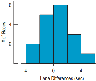
Speed-Skating Comparisons
Mechanics:
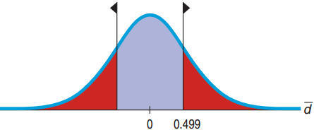
\(n\) = 17 pairs, \(\bar{d}\) = 0.499 sec., \(s_d\) = 2.333 sec.
\[SE\left(\bar{d}\right) = \frac{s_d}{\sqrt{n}} = \frac{2.333}{\sqrt{17}} = 0.5658\]
\[t_{16} = \frac{\bar{d} - 0}{SE\left(\bar{d}\right)} = \frac{0.499}{0.5658} \approx 0.882\]
\[\text{P-value} = 2P(t_{16} > 0.882) = 0.39\]
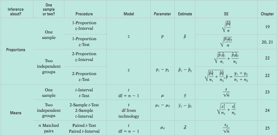
Speed-Skating Comparisons
- Conclusion:
- Events that occur more than a third of the time (P-value = 0.39) are not remarkable.
- I can’t conclude that the observed difference isn’t due simply to random chance. It appears the fans may have interpreted a random fluctuation in the data as favoring one lane. There’s insufficient evidence to declare any lack of fairness.
4-Day vs. 5-Day Mileage
- P-value = 2P(t10 > 2.86) = 0.017
- Since the P-value is small, reject H0.
- Conclude that the change in workweek did lead to a change in average driving mileage. It appears that changing the work schedule may reduce the mileage driven by workers.
- The confidence interval will help determine if there is practical significance.
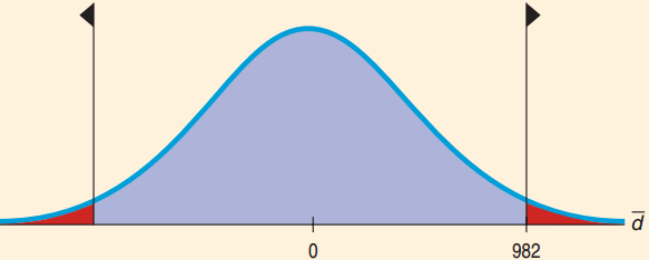
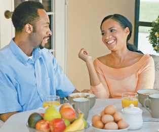
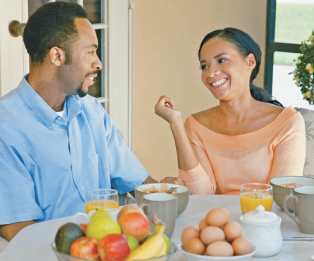
How Much Older is the Husband?
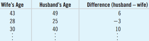
170 couples selected at random provided their ages.
- Goal: Find a confidence interval for the mean difference.
How Much Older is the Husband?
How big a difference is there, on average, between husbands and wives?
- Plan: I want the mean difference in age. Have a random sample of 200 couples with 170 providing their ages. \(n\) = 170
- Model:
- Paired Data Condition: Married couples make a natural pairing.
- Independence Assumption: The survey was randomized.
How Much Older is the Husband?
- Model:
- Nearly Normal Condition: The histogram is unimodal and symmetric.
- The conditions are met, so I can use the Student’s t-model with \(n - 1 = 169\) degrees of freedom and find a paired t-interval.
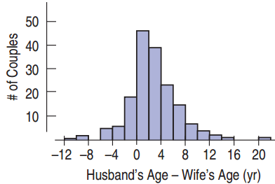
How Much Older is the Husband?
- Mechanics: \(n\) = 170, \(\bar{d}\) = 2.2 years, \(s_d\) = 4.1 years
How Much Older is the Husband?
- Mechanics: \(n\) = 170, \(\bar{d}\) = 2.2 years, \(s_d\) = 4.1 years
\[SE\left(\bar{d}\right) = \frac{s_d}{\sqrt{n}} = \frac{4.1}{\sqrt{170}} = 0.31 \text{ year}\]
\(t_{169}\) = 1.97 (from computer)
\[ME = t^*_{169} \times SE\left(\bar{d}\right) = 1.97 \times 0.31 \approx 0.61\]
- The 95% CI for the difference between the means is 2.2 ± 0.61 = 1.6 to 2.8 years.
How Much Older is the Husband?
- Conclusion: I am 95% confident that husbands are, on average, 1.6 to 2.8 years older than their wives.
Comparing Pairs and No Pairs
Pairing
- With pairing husbands and wives, there was a clear difference in ages. 95% CI: (1.6, 2.8).
Without Pairing
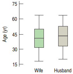
- Without pairing, this would not have been as conclusive.
- From the box plots the difference is hard to detect.
Are CEO Zodiac Signs Uniform?
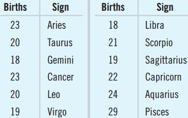
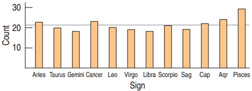
- A survey of 256 randomly selected CEOs’ Zodiac signs
- If uniform, each sign expected to have 256/12 ≈ 21.3 births
- Pisces has more.
- Others have fewer.
- Is the distribution far enough from uniform to conclude the data do not come from a uniform distribution?
Finding Expected Counts
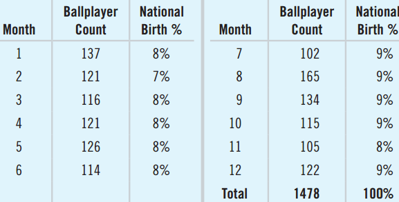
1478 baseball players’ birth months.
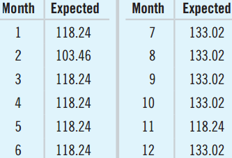
- Find the expected count for each month.
- January: 1478 × 0.08 = 118.24
- February: 1478 × 0.07 = 103.46
Chi-Square P-Values
Baseball Birth Months
- H0: The distribution of baseball player birth months is the same as for the general population.
- HA: The distribution of baseball player birth months is not the same as for the general population.
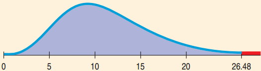
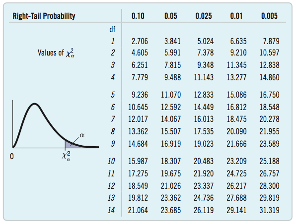
- \(\chi^2_{11} = 26.48\) P-value = 0.0055 (or 0.005 < p < 0.01)
- There’s evidence that major league ballplayers’ birth months have a different distribution from the rest of us.
Zodiac Signs of CEOs
- Plan: I have the zodiac signs of 256 CEOs. Is there a uniform distribution?
- Hypotheses:
- H0: Births are uniformly distributed over zodiac signs.
- HA: Births are not uniformly distributed over zodiac signs.

Zodiac Signs for CEOs
Model
- Counted Data Condition: I have counts of each sign.
- Independence Assumption: This is a convenience sample, but no reason to expect bias with respect to birthdays.
- Expected Cell Frequency Condition: 21.3 \(\geq\) 5.
- The conditions are satisfied. I will use the Chi-Square Goodness-of-Fit Model with 12 – 1 = 11 degrees of freedom.
Zodiac Signs for CEOs
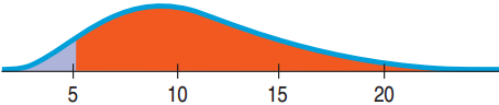
- Mechanics: \(\chi^2_{11} = 5.094\), P-value = 0.926 (from computer)
- Conclusion: If the zodiac signs of CEOs were distributed uniformly, an observed chi-square value of 5.09 or higher would occur about 93% of the time.
- Fail to reject the H0. Conclude that there is no evidence of nonuniform distribution of zodiac signs among CEOs.
Why so big? The Shape of \(\chi^2\)
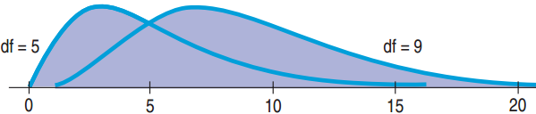
- With df large (more cells), the weighted residuals add up quickly → numerator gets bigger \(\chi^2 = \sum \frac{\left(Obs - Exp\right)^2}{Exp}\)
- Unlike z or t, a larger \(\chi^2\) is more common. It all depends on the df: look at value 10
- The mode of \(\chi^2\) is df – 2.
- The expected value of \(\chi^2\) is df, to the right of the mode due to the right skewed distribution.
- The CEO curve had df = 11, peaks at 9 and mean = 11
Activities of Graduates at Different Colleges
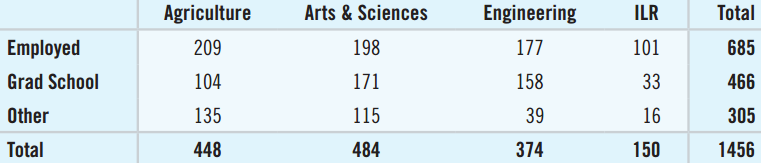
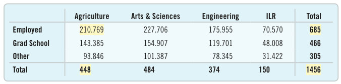
- Are graduates’ activities the same at different colleges within the same university?
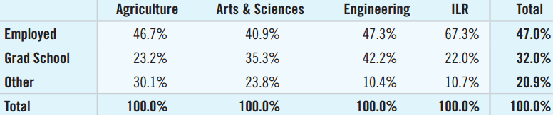
- Class-size differences cloud the table. Proportions may be helpful.
Calculations
Expected Counts?
- 685, or about 47.0%, of the 1456 students who responded to the survey were employed.
- Of the 448 agriculture students, expect 47% of 448 or 210.76 to be employed.
\(\chi^2\) Calculation
- Use the same formula with these observed and expected. df = (R – 1)(C – 1) = (3 – 1)(4 – 1) = 6.
Students’ Choices Same Across Colleges?
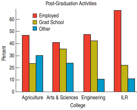
- Model: The bar chart shows how the percents differ.
- Counted Data Condition: I will use the table of counts.
- Independence Assumption: It is not a random sample, but with this large study, most students act independently of the others.
- Expected Cell Frequency Condition: All \(\geq\) 5
- Use the \(\chi^2\)-model with df = 6 and do a chi-square test for homogeneity.
Students’ Choices Same Across Colleges?
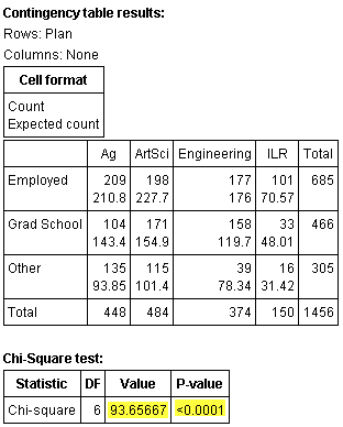
- Mechanics: I used the computer to produce the expected counts, \(\chi^2\), and P-value.
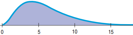
- \(\chi^2 \approx 93.66\)
- P-value < 0.0001
Standardized Residuals for College Grads
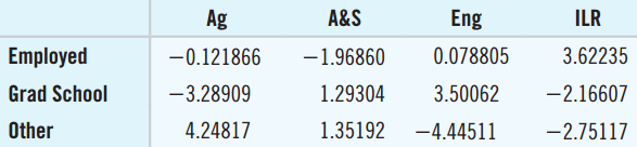
- Engineering students: c is big, far from the expected value
- → They disproportionately go to grad school and not pursue other activities.
- Agriculture students disproportionately pursue other activities.
Hepatitis and Tattoos
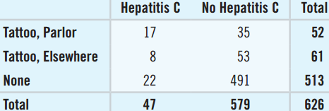
The contingency table shows the results of a study that looked at where people had their tattoo and whether they have Hepatitis C.
- Two categorical variables
- Contingency tables are used to see if one categorical variable is contingent on another.
- Are Hepatitis C and Tattoo Status independent?
Tattoos and Hepatitis
Are Tattoo Status and Hepatitis Status independent?
- Plan: Test for independence. I have a contingency table of 626 patients.
- Hypotheses:
- H0: Tattoo Status and Hepatitis Status are independent.
- HA: Tattoo Status and Hepatitis Status are not independent.

Tattoos and Hepatitis
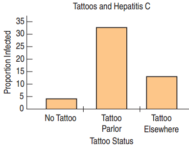
- Model: The bar chart suggests a difference in Hepatitis C based on tattoo status.
- Counted Data Condition: I have counts of individuals categorized on two variables.
- Independence Assumption: Not SRS, but likely independent.
Tattoos and Hepatitis
- Model: (Continued)
- Expected Cell Frequency Condition: Two expected counts < 5.
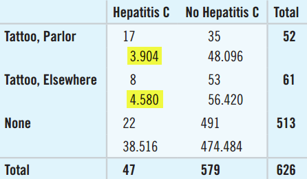
- Not all the assumptions are met, but I will carefully go ahead with the chi-square test for independence with df = (3 – 1) × (2 – 1) = 2. I will check the residuals carefully.
Tattoos and Hepatitis C
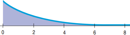
- Mechanics: With df = 2 the \(\chi^2\) graph looks very different.
- Use computer just like with Homogeneity.
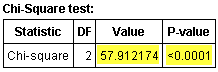
- \(\chi^2 = 57.91\), P-value < 0.0001
Examining the Residuals
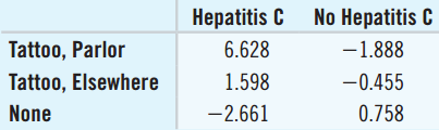
- Parlor/Hepatitis C residual is large positive. More Hepatitis C from those with tattoos from parlors than expected.
- None/Hepatitis C residual large negative. Less Hepatitis C from those without tattoos than expected.
- Cell counts small for Parlor/Hepatitis C. We should report this as a warning, or rethink the data.
- How can we increase cell counts?
Combining Groups
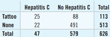
- Combining all those with tattoos gives large enough counts.
- New \(\chi^2 = 42.42\) (df = 1)
- New P-value < 0.0001
- We conclude that Tattoo Status and Hepatitis C Status are not independent.
- We are concerned, but need more evidence to suggest that tattoo parlors are a problem.
Race and Traffic Stops
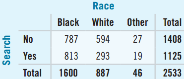
- Data were collected on drivers’ race and whether they were searched when an officer stopped them.
- What test to decide if race is a factor in vehicle searches?
- Two categorical variables: Race and Search.
- Chi-Square test for independence.
- H0: Race and Search are independent.
- HA: Race and Search are not independent.
Chi-Square Mechanics
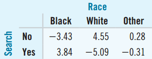
Find the df, expected frequency for Black drivers who were stopped, that cell’s component of \(\chi^2\), and its residual.
- df = (2 – 1)(3 – 1) = 2
- Expected Frequency: \(\dfrac{1125}{2533} \times 1600 \approx 710.62\)
- \(\chi^2\) Contribution: \(\dfrac{\left(813 - 710.62\right)^2}{710.62} \approx 14.75\)
- S.Residual: \(\dfrac{\left(813 - 710.62\right)}{\sqrt{710.62}} \approx 3.84\)
Race and Traffic Stop Searches
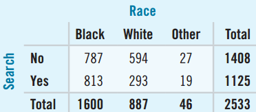
- P-value < 0.0001
- There is strong evidence to conclude that police decisions to search are associated with race.
- Large residuals for Whites suggests that police search Whites less than independence would predict.
- It appears that Black drivers’ cars are searched more often.