Quantitative Methods

Lecture 16

Serena DeStefani

2020-08-04

Quantitative Methods

Serena DeStefani – Lecture 16 – 8/4/2020

Announcements: Final Exam

• Non-cumulative, 2&1/2 hours long, as the midterm
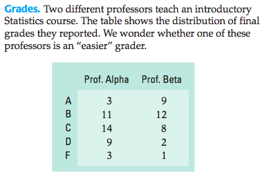
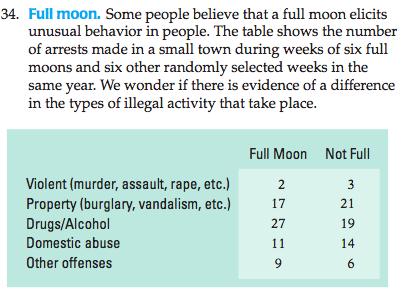
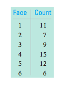
• Same format as HWs, focus on inference (no CH 15/16)
• Problems (can be both tests and CIs) on inference for means, proportions, regression, one chi-square test, and questions about Analysis of Variance (I will give you the ANOVA table)

Chapter 24

Comparing Counts

24.1

Goodness-of-Fit Test

Finding Expected Counts

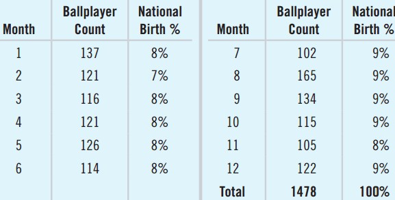
1478 baseball players’ birth months.

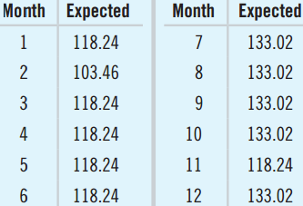
• Find the expected count for each month.

. . .

• January: 1478 × 0.08 = 118.24
• February: 1478 × 0.07 = 103.46

Assumptions and Conditions

Counted Data Condition

• The values in each cell are counts.
• Doesn’t work with percents, proportions, or measurements

Independence Assumption

• The counts in each cell must be independent of each other.
• For random samples, we can generalize to the entire population.

Assumptions and Conditions (Continued)

Sample Size Assumption

• Expected counts for each cell ≥ 5.
• This is called the Expected Cell Frequency Condition.

If the assumptions and conditions are met, we can perform a Chi-Square Test for Goodness-of-Fit.

Chi-Square Calculations

• Interested in difference between observed and expected: residuals.
• Make positive by squaring them all.
• Get relative sizes of the residuals by dividing them by the expected counts.

\[\chi^2 = \sum \frac{\left(Obs - Exp\right)^2}{Exp}\]

• This is a Chi-Square Model with df = n – 1.
• n is the number of categories, not the sample size.

Chi-Square P-Values

Baseball Birth Months

• H₀: The distribution of baseball player birth months is the same as for the general population.
• H_A: The distribution of baseball player birth months is not the same as for the general population.

• \(\chi^2_{11} = 26.48\)   P-value = 0.0055 (or 0.005 < p < 0.01)
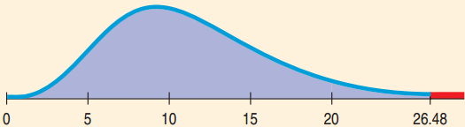
• There’s evidence that major league ballplayers’ birth months have a different distribution from the rest of us.

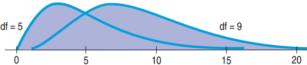
Why so big? The Shape of \(\chi^2\)

• With df large (more cells), the weighted residuals add up quickly → numerator gets bigger   \(\small\chi^2 = \sum \frac{(Obs - Exp)^2}{Exp}\)
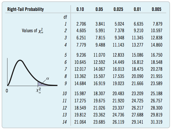
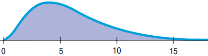
• Unlike z or t, a larger \(\chi^2\) is more common. It all depends on the df: look at value 10
• The mode of \(\chi^2\) is df – 2.
• The expected value of \(\chi^2\) is df, to the right of the mode due to the right skewed distribution.
• The CEO curve had df = 11, peaks at 9 and mean = 11

24.2

Chi-Square Test for Homogeneity

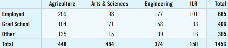
Activities of Graduates at Different Colleges

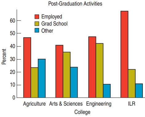
• Are graduates’ activities the same at different colleges within the same university?
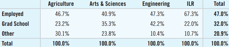
• Class-size differences cloud the table. Proportions may be helpful.

Test for Homogeneity

• More than two proportions to compare, so we cannot use the two-proportion z-test.
• Generalize to the chi-square test for homogeneity.
• Same mechanics as goodness-of-fit, different hypotheses and conclusions.
• Chi-square test for homogeneity asks if the distribution is the same for different groups.
• The test looks for differences large enough to step beyond what we might expect from random sample-to-sample variation

Assumptions and Conditions

Same as Goodness-of-Fit

• Counted Data Condition: Always use counts, not proportions, percents, or measurements.
• Independence Assumption: Need randomization to generalize to the population.
• Expected Cell Frequency Condition: All expected counts should be at least 5.

Calculations

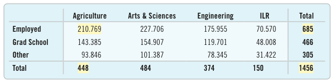
Expected Counts?

• 685, or about 47.0%, of the 1456 students who responded to the survey were employed.
• Of the 448 agriculture students, expect 47% of 448 or 210.76 to be employed.

\(\chi^2\) Calculation

• Use the same formula with these observed and expected. df = (R – 1)(C – 1) = (3 – 1)(4 – 1) = 6.

Students’ Choices Same Across Colleges?

• Plan: I have a table of counts from the college’s class of 2011.
• Hypotheses:
  • H₀: Students’ post-graduation activities are distributed in the same way for all four colleges.
  • H_A: Students’ plans do not have the same distribution.

Students’ Choices Same Across Colleges?

• Model: The bar chart shows how the percents differ.
  • Counted Data Condition: I will use the table of counts.
  • Independence Assumption: It is not a random sample, but with this large study, most students act independently of the others.
  • Expected Cell Frequency Condition: All ≥ 5
• Use the \(\chi^2\)-model with df = 6 and do a chi-square test for homogeneity.

Students’ Choices Same Across Colleges?

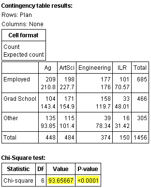
• Mechanics: I used the computer to produce the expected counts, \(\chi^2\), and P-value.

• \(\chi^2 \approx 93.66\)
• P-value < 0.0001

Students’ Choices Same Across Colleges?

• Conclusion: The P-value is very small, so I reject the null hypothesis.
• I conclude that there’s evidence that the post-graduation activities of students from these four colleges don’t have the same distribution.

24.3

Examining the Residuals

Examining the Residuals

• After rejecting H₀, we wonder where things differed.
• The residuals can be helpful.
• Even better, standardized residuals:

\[c = \frac{Obs - Exp}{\sqrt{Exp}}\]

• Standardized residuals are like z-scores.
• Tells us how far the observed is above or below the expected.

Standardized Residuals for College Grads

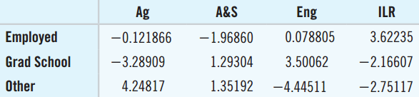
• Engineering students: c is big, far from the expected value
• → They disproportionately go to grad school and do not pursue other activities.
• Agriculture students disproportionately pursue other activities.

24.4

Chi-Square Test of Independence

Hepatitis and Tattoos

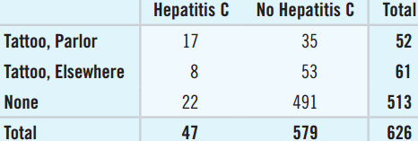
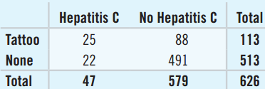
The contingency table shows the results of a study that looked at where people had their tattoo and whether they have Hepatitis C.

• Two categorical variables
• Contingency tables are used to see if one categorical variable is contingent on another.
• Are Hepatitis C and Tattoo Status independent?

Independence

• Two events are independent if P(A|B) = P(A).
• If Tattoo Status and Hepatitis C are independent, we would expect the proportions of “positive” to be the same for the three levels of Tattoo Status.
• Same criterion as homogeneity
• The nuances of homogeneity and independence statements are different.
• Same distribution vs. independent

Assumptions and Conditions

• Counted Data Condition: Always use counts, not proportions, percents, or measurements.
• Independence Assumption: The data were collected independently.
• Expected Cell Frequency Condition: All expected counts at least 5.
• 10% Condition: Data come from a random sample of less than 10% of the population.

Tattoos and Hepatitis

• Model: (Continued)
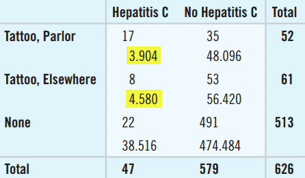
  • Expected Cell Frequency Condition: Two expected counts < 5.
• Not all the assumptions are met, but I will carefully go ahead with the chi-square test for independence with df = (3 – 1) × (2 – 1) = 2. I will check the residuals carefully.

Tattoos and Hepatitis C

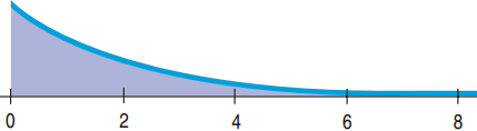
• Mechanics: With df = 2 the \(\chi^2\) graph looks very different.
• Use computer just like with Homogeneity.

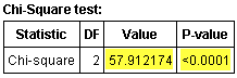
• \(\chi^2\) = 57.91, P-value < 0.0001

Tattoos and Hepatitis C

• Conclusion: With P-value < 0.0001, reject H₀. Tattoo Status and Hepatitis Status are not independent.
• Since the expected counts are < 5, I need to check that the cells with small expected counts did not influence the results too greatly.

Examining the Residuals

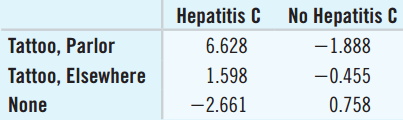
• Parlor/Hepatitis C residual is large positive. More Hepatitis C from those with tattoos from parlors than expected.
• None/Hepatitis C residual large negative. Less Hepatitis C from those without tattoos than expected.
• Cell counts small for Parlor/Hepatitis C. We should report this as a warning, or rethink the data.
• How can we increase cell counts?

Combining Groups

• Combining all those with tattoos gives large enough counts.
• New \(\chi^2\) = 42.42 (df = 1)
• New P-value < 0.0001
• We conclude that Tattoo Status and Hepatitis C Status are not independent.
• We are concerned, but need more evidence to suggest that tattoo parlors are a problem.

Race and Traffic Stops

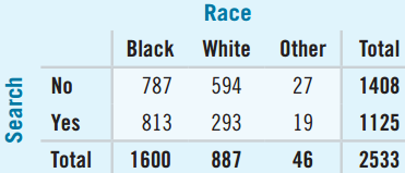
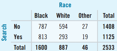
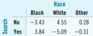
• Data were collected on drivers’ race and whether they were searched when an officer stopped them.
• What test to decide if race is a factor in vehicle searches?
• Two categorical variables: Race and Search.
• Chi-Square test for independence.
  • H₀: Race and Search are independent.
  • H_A: Race and Search are not independent.

Chi-Square Mechanics

Find the df, expected frequency for Black drivers who were stopped, that cell’s component of \(\chi^2\), and its residual.

• df = (2 – 1)(3 – 1) = 2
• Expected Frequency: \(\ \dfrac{1125}{2533} \times 1600 \approx 710.62\)
• \(\chi^2\) Contribution: \(\ \dfrac{\left(813 - 710.62\right)^2}{710.62} \approx 14.75\)
• S.Residual: \(\ \dfrac{\left(813 - 710.62\right)}{\sqrt{710.62}} \approx 3.84\)

Race and Traffic Stop Searches

• P-value < 0.0001
• There is strong evidence to conclude that police decisions to search are associated with race.
• Large residuals for Whites suggests that police search Whites less than independence would predict.
• It appears that Black drivers’ cars are searched more often.

Chi-Square and Causation

• Just like correlation, rejecting H₀ for a chi-square test does not imply causation.
  • Does having Hepatitis C cause a craving to get a tattoo?
  • Maybe there is a lurking variable.
  • Is there a subculture that tends to have both?
  • Just state independence, not causation.

What Can Go Wrong?

Don’t use chi-square methods unless you have counts.

• Convert percents and proportions back to counts.

Beware large samples.

• There are no confidence intervals to see “how not independent” the categories are. Rarely are categories perfectly independent.

Don’t say that one variable “depends” on the other just because they’re not independent

• “Depends” suggests causation. Just state that the categories are “not independent” or are “associated.”

Summary: Chi-Square test for count data

• A single basis of classification: Goodness of fit
• df: n – 1, where n is the number of categories

• Two variables, more than one population: Homogeneity

• Two variables, one population: Independence

Review: Chi-Square test for count data

Review: Chi-Square test for count data

Review: Chi-Square test for count data

Chapter 25

Inferences on Regression

25.1

The Population and the Sample

Review: The Linear Model

Fat and Protein at Burger King

• The correlation is 0.76.
• This indicates a strong linear fit, but how do we choose the line?
• The line should be “closest” to the points.

Review: The Residuals

• \(\hat{y}\) is the value on the line
• It is called the predicted value.
• For each point \((x, y)\) look at the point \((x, \hat{y})\) on the line with the same x-coordinate.
• The residual is defined by \(\ y - \hat{y}\)
• The residual is the difference between the observed value and the predicted value.

Review: The Residuals

Residual:

• Observed – Predicted
• Points above the line have positive residuals
• Points below the line have negative residuals.
• This line gives the average fat content expected for a given amount of protein.

Review: The Line of Best Fit

• The best fitting line will have small residuals.
• High negative residuals are just as “bad” as high positive residuals.
• Squaring all residuals makes them all positive.
• The line of best fit is the line for which the sum of the squares of the residuals is the smallest, also called the least squares line.

Waist size and %Body Fat

• Can we predict the amount of %Body-Fat from Waist size?
• We can take a sample of men, measure %Body-Fat and Waist size for each, and run a regression
• For each value of Waist size I will have maybe one value, maybe one or two values of %Body-Fat
• But what happens if I think about the whole population of men?
• For each value of Waist Size I will have many different values of %Body-Fat!

• How will they be distributed?

Many Distributions for Regression

• We saw how to build a single distribution for means and proportions.
• How do we translate this concept to regression?
• If we think about the population, for each value of waist there are different values of %Body-Fat
• With regression, for each value of x there is a different distribution for y.
• This model assumes that for each x, the mean of the y’s is on the regression line.

Sample vs. Model Regression

Sample: \(\ \hat{y} = b_0 + b_1 x\)

• This gives a prediction for y based on the sample.

Model: \(\ \mu_y = \beta_0 + \beta_1 x\)

• \(\beta_0\) = y-intercept for the model
• \(\beta_1\) = slope for the model
• The model assumes that for every value of x, the mean of all the y’s lies on the line.

Error

\[\mu_y = \beta_0 + \beta_1 x\]

• The model predicts the mean of y for each x, but misses the actual (observed) individual values of y.
• The error, \(\varepsilon\), is the amount the line misses the value of y.
• \(\varepsilon\) is analogous to e, the residual: \(\ e = y - \hat{y}\)
• We want to define a new equation that incorporates the error:

\[y = \beta_0 + \beta_1 x + \varepsilon\]

• This new equation gives the exact value of each of the observed y’s.

How Good is the Model?

• The least squares regression line \(\ \hat{y} = b_0 + b_1 x\ \) obtained from the sample gives estimates for the model.
  • \(b_0\) is an estimate for \(\beta_0\).
  • \(b_1\) is an estimate for \(\beta_1\).

• Challenge: How good are these estimates?

25.2

Assumptions and Conditions

Assumption and Conditions for Regression

To make inferences about the regression line we need:

• The Straight Enough Condition: We needed to use the line.
• Additional assumptions and conditions related to inference
• Order in which we check conditions is important

1. Linearity Assumption

Straight Enough Condition

• Does the scatterplot look relatively straight?
• Don’t draw the line. It can fool you.
• Look at scatterplot of the residuals.
  • Should have horizontal direction
  • Should not have a pattern
• If straight enough, check the other assumptions.
• If not straight, stop or re-express.

2. Independence Assumption

Errors (\(\varepsilon\)’s) must be independent of each other.

• Check residuals plot.
  • Shouldn’t have clumps, trends, or a pattern.
  • Should look very random.
• For x = time, plot residuals vs. residuals one step later.
  • Should look very random.
• To make inferences about the population, the sample must be representative.

3. Equal Variance Assumption

Variability of y same for all x.

• Does the Plot Thicken? Condition: Spread along the line should be nearly constant.
• “Fan Shape” is bad →
• Standard Deviation of Residuals, \(s_e\), will be used for CI and Hypothesis Tests. This requires same variance for each x.

4. Normal Population Assumption

The errors for each fixed x must follow the Normal model.

• Good enough to use the Nearly Normal Condition – but check for Outliers. Look at the histogram.
• With large sample sizes, the Nearly Normal Condition is usually satisfied.

Crater Age vs. Size

Are the Assumptions and Conditions Satisfied?

• Linearity Assumption: Scatterplot looks straight enough (after re-expressing).
• Independence Assumption: Need to understand the science better to determine this

Crater Age vs. Size

Are the Assumptions and Conditions Satisfied?

• Does the Plot Thicken? The residual plot shows the variances of the residuals are pretty constant.

Crater Age vs. Size

Are the Assumptions and Conditions Satisfied?

• Nearly Normal Condition: The plots show some left skewness.
• The violations are not too severe but I will be cautious about my conclusions.

Steps for Checking Conditions

1. Check Straight Enough Condition with scatterplot.
2. Fit regression, find predicted values and residuals.
3. Make residuals scatterplot and check for thickening, bends, and outliers.
4. For x = time, use residuals plot to check for independence.
5. Check the Nearly Normal Condition with a histogram and Normal plot of residuals.
6. If all conditions reasonably satisfied, proceed with inference.

Body Fat and Waist Size

What is the relationship between body fat and waist size in men?

• Plan: I have measurements on 250 adult males.
• Model:
  • Straight Enough Condition: The scatterplot looks very straight.

Body Fat and Waist Size

• Model:
  • Independence Assumption: No reason to think that one man’s fat influences another’s.
  • Does the Plot Thicken? Condition: Neither the original scatterplot nor the residuals show changing variances.

Body Fat and Waist Size

• Mechanics: Computer Output:

• The estimated regression equation is:

\[\widehat{\%Body\ Fat} = -42.73 + 1.70\ Waist\]

Body Fat and Waist Size: R code

body_fat <- read.csv("Body_fat_complete.csv")
reg_bf <- lm(Pct.BF ~ waist, body_fat)
summary(reg_bf)

• The estimated regression equation is: \(\ \widehat{\%Body\ Fat} = -42.73 + 1.70\ Waist\)

Body Fat and Waist Size

• Conclusion:
  • R² = 67.8%. Waist size accounts for about 2/3 of the variation in %Body Fat.
  • Slope = 1.7. %Body Fat increases about 1.7% for each inch increase in body fat, on average.
  • Standard Error for slope = 0.07, smaller than the slope. The estimate is reasonably precise.

25.3

Intuition About Regression Inference

Sample-to-Sample Variation of Slope and Intercept

• Each sample will produce its own slope (\(b_1\)) and intercept (\(b_0\)).
• The expected value of \(b_1\) should be \(\beta_1\).
• What is the standard deviation of all possible \(b_1\)’s?
• What factors influence this standard deviation?
• What factors influence the standard deviation of \(b_0\)?

Spread Around the Line

• Less scatter along line → Slope more consistent
• Residual Standard Deviation \(s_e\) measures this scatter.

\[s_e = \sqrt{\frac{\sum \left(y - \hat{y}\right)^2}{n - 2}}\]

Spread of the x’s, Sample Size

• Larger \(s_x\) (SD in x) → More stable regression

• Larger Sample Size → More stable regression

Standard Error for the Slope

\[SE\left(b_1\right) = \frac{s_e}{\sqrt{n - 1}\ s_x}\]

• From the formula, \(SE(b_1)\) increases with \(s_e\) (SD of residuals) and decreases with \(s_x\) (SD of x)
• If we subtract \(\beta_1\) from \(b_1\) and divide by \(SE(b_1)\), the result is a Student’s t-model with df = n – 2.

\[\frac{b_1 - \beta_1}{SE\left(b_1\right)} \sim t_{n-2}\]

Sampling Distribution for Regression Slopes

• When the conditions are met, \(\ t = \dfrac{b_1 - \beta_1}{SE\left(b_1\right)}\ \) follows Student’s t-model with df = n – 2.

• Estimate of the standard error:

\[SE\left(b_1\right) = \frac{s_e}{\sqrt{n - 1}\ s_x}, \quad s_e = \sqrt{\frac{\sum \left(y - \hat{y}\right)^2}{n - 2}}\]

Standard Errors for Craters

• Verify the standard error and t-ratio for the slope.
• H₀: No linear association: \(\beta_1 = 0\)

\[SE\left(b_1\right) = \frac{0.6362}{\sqrt{39 - 1} \times 1.57682} = 0.0655 \qquad t_{37} = \frac{0.526674 - 0}{0.0655} = 8.04\]

What About the Intercept?

\[\frac{b_0 - \beta_0}{SE\left(b_0\right)} \sim t_{n-2}\]

• The intercept is rarely of interest.
• Hypotheses and CI are usually about the slope only.

25.4

Regression Inference

Testing for \(\beta_1\)

• If no linear association, \(\beta_1 = 0\)
• H₀: \(\beta_1 = 0\)

\[t_{n-2} = \frac{b_1 - 0}{SE\left(b_1\right)}\]

• For the %Body Fat and Waist data:

\[\frac{1.7 - 0}{0.0743} \approx 22.9 \qquad \text{P-value} < 0.0001\]

• Very unlikely to have such a high \(b_1\) if \(\beta_1 = 0\)
• IF no association in population, sample is unlikely

Confidence Interval for \(\beta_1\)

• The hypothesis test for %Body Fat and Weight told us what we already know.
• A confidence interval is needed.

\[b_1 \pm t^*_{n-2} \times SE(b_1)\]

• For %Body Fat and Weight:
  • 1.7 ± 1.97 × 0.074 = (1.55%, 1.85%)
• With 95% confidence the slope of the line for %Body Fat and Weight is between 1.55% and 1.85%.

Craters: Interpreting Regression

• What does the regression model tell us?
  • \(\widehat{\log Diam}\) = 0.358 + 0.527 logAge
  • P-value ≤ 0.0001, reject H₀.
  • Conclude that, on average, the older the crater is the larger it tends to be.

Craters: Interpreting Regression

• What does the regression model tell us?
  • The model accounts for 63.6% of the variation in logDiam.
  • The evidence of correlation does not imply bigger craters were more common long ago. Maybe only the big ones survive erosion.

When Will the Ice Break?

Contest since 1917 on guessing when the tripod will fall through the Alaskan ice.

Ice Breakup Date Per Year

Is there sufficient evidence to claim that the ice breakup times are changing? If so, how fast?

• Plan: I have 95 years of data. The slope might indicate climate change.
• Hypotheses:
  • H₀: \(\beta_1 = 0\)
  • H_A: \(\beta_1 \neq 0\)

Ice Breakup Date Per Year

• Model:
• Straight Enough Condition: No bends in scatterplot.
• Independence Assumption: Time series, so be careful. A little up and down. Not a random sample, so cannot extend beyond this year.

Ice Breakup Date Per Year

• Model:
• Does the Plot Thicken? Condition: No obvious trends in the residual plot.
• Nearly Normal, Outlier Condition: Histogram of residuals unimodal, symmetric with no outliers
• The sampling distribution of the slope is modeled by Student’s t (df = 93).
• I’ll do a regression slope t-test.

Ice Breakup Date Per Year

• Mechanics:
• \(\widehat{Date}\) = 128.581 - 0.068 YearSince1900
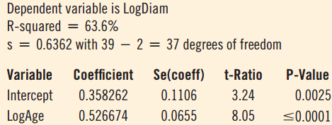
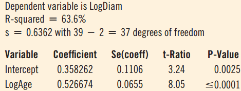
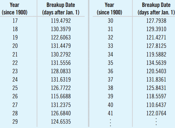
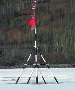
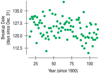
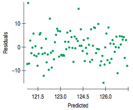
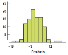
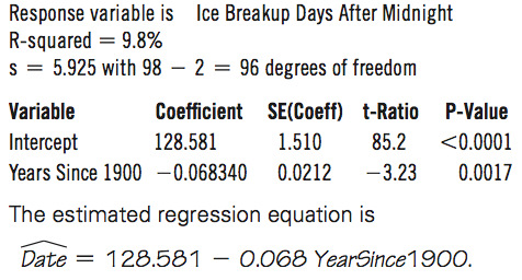
• Conclusion: P-value = 0.0017, the association is unlikely to occur by chance, even though R-squared is weak. There is strong evidence the ice breakup is occurring earlier.
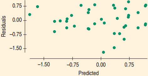
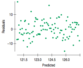
• Oscillation of residuals raised concerns.

Ice Breakup Date Per Year

• Create a Confidence Interval for the Slope
  • – 0.068 ± (1.985)(0.0212) = (– 0.11, – 0.03)
• Interpretation: I am 95% confident that the ice has been breaking up, on average, between 0.03 days (about 40 minutes) and 0.11 days (about 3 hours) earlier each year since 1917.

What is Causing the Early Ice Breakup?

• Based on the regression conclusions can we say that global warming is causing the early ice breakup?

• No! Causation cannot be concluded from association.
• Maybe it is global warming.
• Maybe it is from the area’s human activities warming up the water below.

25.5

Standard Errors for Predicted Values

Two Prediction Questions

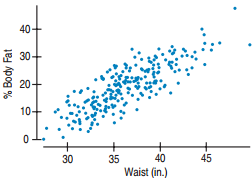
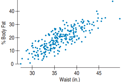
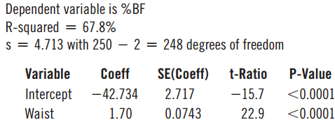
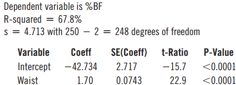
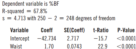
1. Predict the %Body Fat of a man with waist 38 in.
   • Notice the prediction is for a single man.
2. Predict the mean %Body Fat for all men with waist 38 in.
   • This prediction is for a mean.

• Both have the same prediction: \(\ \hat{y}_\nu = b_0 + b_1 x_\nu\)
• The confidence intervals: \(\ \hat{y}_\nu \pm t^*_{n-2} \times SE\)
• The standard errors (SE) will differ.

Standard Error for the Mean

\[SE(\hat{\mu}_\nu) = \sqrt{SE^2(b_1) \times \left(x_\nu - \bar{x}\right)^2 + \frac{s_e^2}{n}}\]

• \(SE(\hat{\mu}_\nu)\) increases as \(SE(b_1)\) increases.
• \(SE(\hat{\mu}_\nu)\) increases as \(x_\nu\) strays from the mean of the x’s.
• \(SE(\hat{\mu}_\nu)\) increases as \(s_e\) increases.
• \(SE(\hat{\mu}_\nu)\) decreases as n increases.

Standard Error for a Single Prediction

\[SE(\hat{y}_\nu) = \sqrt{SE^2(b_1) \times \left(x_\nu - \bar{x}\right)^2 + \frac{s_e^2}{n} + s_e^2}\]

• Individual values vary more than means.
• \(SE(\hat{y}_\nu)\) has the extra positive term \(s_e^2\).
• When looking at a computer output, remember the smaller SE is for the predicted mean value and the larger is for the predicted individual value.

25.6

Confidence Intervals for Predicted Values

Confidence Interval for the Mean

Find the 95% CI for the mean %Body Fat of all men who have 38 inch waists.

• \(s_e = 4.713,\ n = 250,\ SE(b_1) = 0.074,\ \bar{x} = 36.3,\ x_\nu = 38\)

\[\hat{y}_\nu = b_0 + b_1 x_\nu \qquad SE(\hat{\mu}_\nu) = \sqrt{SE^2(b_1) \times \left(x_\nu - \bar{x}\right)^2 + \frac{s_e^2}{n}}\]

\[\hat{y}_\nu = -42.7 + 1.7(38) = 21.9\%\]

\[SE(\hat{\mu}_\nu) = \sqrt{0.074^2 \times \left(38 - 36.3\right)^2 + \frac{4.713^2}{250}} = 0.32\%\]

Confidence Interval for the Mean

• \(t^*_{248} = 1.97\)
• ME = 1.97 × 0.32 = 0.63%
• CI: 21.9% ± 0.63%
• I am 95% confident that the mean %Body Fat for men with a 38 inch waist is 21.9% ± 0.63%.

Prediction Interval for an Individual

Find a prediction interval for the %Body Fat for an individual man with a 38-inch Waist.

\[SE(\hat{y}_\nu) = \sqrt{0.074^2 \times \left(38 - 36.3\right)^2 + \frac{4.713^2}{250} + 4.713^2} = 4.72\%\]

• ME = 1.97 × 4.72 = 9.30%
• The prediction interval is: 21.9% ± 9.30%.
• There is a 95% chance that this interval captures the true %Body Fat of a randomly selected man with a 38-inch waist.

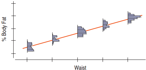
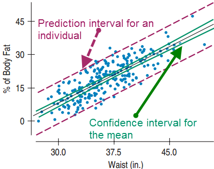
Visualizing the Two Intervals

• The prediction interval for the individual is much wider than the confidence interval for the mean.

What Can Go Wrong?

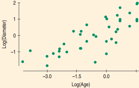
Don’t fit a linear regression to data that aren’t straight.

• Stop here or try re-expressing if not straight.

Watch out for the plot thickening.

• If the points fan out, then the standard deviations are not constant. Don’t perform regression analysis.

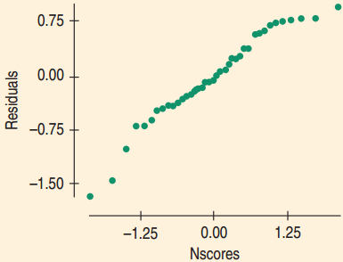
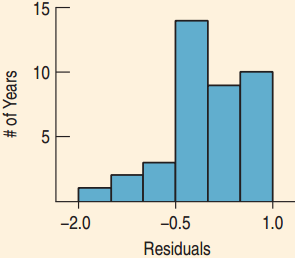
Make sure the errors are Normal.

• Check the histogram and normal probability plot. Need Normal to invoke the CLT.

What Can Go Wrong?

Watch out for extrapolation.

• The model can fail for x-values that are far from the mean of the x’s.

Watch out for influential points and outliers.

• Like other analyses, regression can be strongly influenced by outliers.

Watch out for one-tailed tests.

• Software conducts two-tailed tests for regression. If you need one tail, divide the P-value by 2.

Chapter 28

Multiple Regression

28.1

What is Multiple Regression?

Just Do It

• The method of least squares can be expanded to include more than one predictor. The method is known as multiple regression.
• For simple regression we found the Least Squares solution, the one whose coefficients made the sum of the squared residuals as small as possible.
• For multiple regression, we’ll do the same thing, but this time with more coefficients.

Just Do It (cont.)

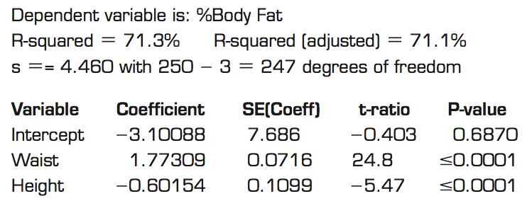
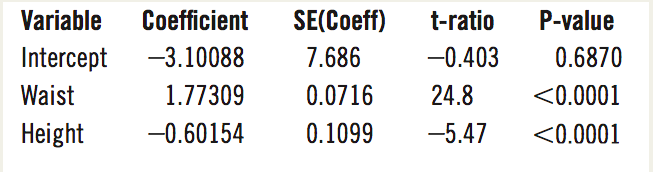
You should recognize most of the numbers in the following example (%body fat) of a multiple regression table. Most of them mean what you expect them to.

So What’s New?

• The meaning of the coefficients in the regression model has changed in a subtle but important way.
• Multiple regression is an extraordinarily versatile calculation, underlying many widely used Statistics methods.
• Multiple regression offers our first glimpse into statistical methods that use more than two quantitative variables.

28.2

Interpreting Multiple Regression Coefficients

What Multiple Regression Coefficients Mean

• We said that height might be important in predicting body fat in men.
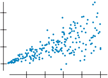
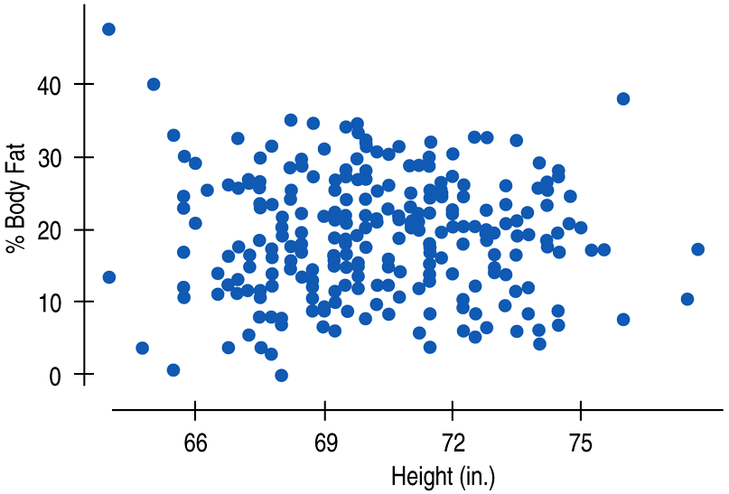
• What’s the relationship between %body fat and height in men? Here’s the scatterplot:

What Multiple Regression Coefficients Mean (cont.)

• It doesn’t look like height tells us much about %body fat. Or does it?
• The coefficient of height in the multiple regression model was statistically significant, so it did contribute to the multiple regression model.
• How can this be?
  • The multiple regression coefficient of height takes account of the other predictor (waist size) in the regression model.

What Multiple Regression Coefficients Mean (cont.)

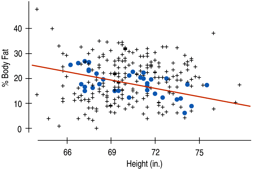
For example, when we restrict our attention to men with waist sizes between 36 and 38 inches (points in blue), we can see a relationship between %body fat and height:

What Multiple Regression Coefficients Mean (cont.)

So, overall there’s little relationship between %body fat and height, but when we focus on particular waist sizes there is a relationship.

• This relationship is conditional because we’ve restricted our set to only those men with a certain range of waist sizes.
• For men with that waist size, an extra inch of height is associated with a decrease of about 0.60% in body fat.
• If that relationship is consistent for each waist size, then the multiple regression coefficient will estimate it.

What Multiple Regression Coefficients Mean (cont.)

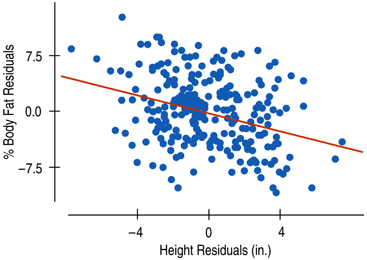
The following partial regression plot shows the coefficient of height in the regression model has a slope equal to the coefficient value in the multiple regression model:

28.3

The Multiple Regression Model - Assumptions and Conditions

The Multiple Regression Model

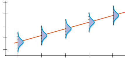
For a multiple regression with k predictors, the model is:

\[y = \beta_0 + \beta_1 x_1 + \beta_2 x_2 + \ldots + \beta_k x_k + \varepsilon\]

The assumptions and conditions for the multiple regression model sound nearly the same as for simple regression, but with more variables in the model, we’ll have to make a few changes.

Assumptions and Conditions

Linearity Assumption:

• Straight Enough Condition: Check the scatterplot for each candidate predictor variable – the shape must not be obviously curved or we can’t consider that predictor in our multiple regression model.

Independence Assumption:

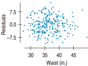
• Randomization Condition: The data should arise from a random sample or randomized experiment. Also, check the residuals plot - the residuals should appear to be randomly scattered.

Assumptions and Conditions (cont.)

Equal Variance Assumption:

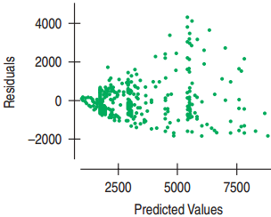
• Does the Plot Thicken? Condition: Check the residuals plot – the spread of the residuals should be uniform.

Assumptions and Conditions (cont.)

Normality Assumption:

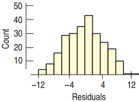
• Nearly Normal Condition: Check a histogram of the residuals – the distribution of the residuals should be unimodal and symmetric, and the Normal probability plot should be straight.

Assumptions and Conditions (cont.)

Summary of the checks of conditions in order:

1. Check the Straight Enough Condition with scatterplots of the y-variable against each x-variable.
2. If the scatterplots are straight enough, fit a multiple regression model to the data.
3. Find the residuals and predicted values.
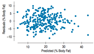
4. Make and check a scatterplot of the residuals against the predicted values. This plot should look patternless.

Assumptions and Conditions (cont.)

Summary of the checks of conditions in order:

5. Think about how the data were collected. Randomization? Representative? Plot residuals against time - patterns?
6. If the conditions check out this far, feel free to interpret the regression model and use it for prediction.
7. If you wish to test hypotheses about the coefficients or about the overall regression, then make a histogram and Normal probability plot of the residuals to check the Nearly Normal Condition.

Example: Multiple Regression Step-By-Step

How should we model %Body Fat in terms of Height and Waist size?

Example: Multiple Regression Step-By-Step

Variables – Name the variables, report the W’s, and specify the questions of interest:

• Have body measurements on 250 adult males from BYU Human Performance Research Center.
• Want to understand relationship between %Body Fat, Height, and Waist size.

Example: Multiple Regression Step-By-Step

Plan – Think about the assumptions and check the conditions.

Straight Enough Condition:

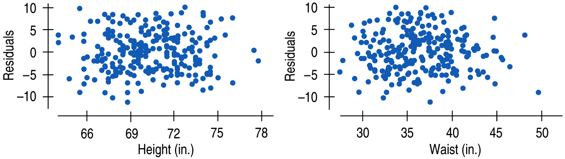
• no obvious bend, scatterplot residuals

Independence Assumption:

• data presented as representative of male population in U.S.

Does the Plot Thicken?

• no obvious changes in the spread

Example: Multiple Regression Step-By-Step

Plan – Think about the assumptions and check the conditions.

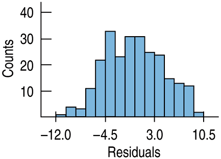
Nearly Normal Condition, Outlier Condition:

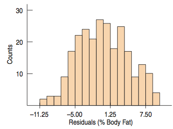
• A histogram of the residuals is unimodal and symmetric.

Example: Multiple Regression Step-By-Step

Plan – Think about the assumptions and check the conditions.

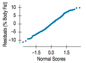
Nearly Normal Condition, Outlier Condition:

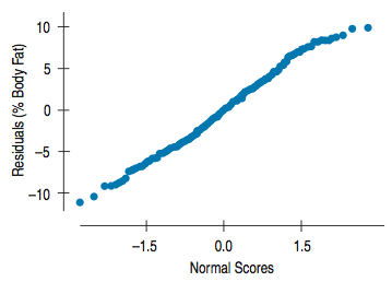
• The Normal probability plot of the residuals is reasonably straight:
• Under these conditions a full multiple regression analysis is appropriate.

Example: Multiple Regression Step-By-Step

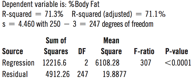
Mechanics – Computer output:

Example: Multiple Regression Step-By-Step

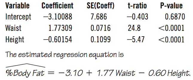
Mechanics

Example: Multiple Regression Step-By-Step

Interpretation

• The R² for the regression is 71.3%.
• Waist size and Height together account for about 71% of the variation.

Example: Multiple Regression Step-By-Step

Interpretation

• Each inch in Waist size is associated with about a 1.77 increase in %Body Fat among men who are of a particular Height
• Each inch of Height is associated with a decrease in %Body Fat of about 0.60 among men with a particular Waist size.

Example: Multiple Regression Step-By-Step

Interpretation

• The standard errors for the slopes of 0.07 (Waist) and 0.11 (Height) are both small compared with the slopes themselves
• → looks like the coefficient estimates are fairly precise.

Example: Multiple Regression Step-By-Step

Interpretation

• The residuals have a standard deviation of 4.46%, which gives an indication of how precisely we can predict %Body Fat with this model.