Quantitative Methods

Lecture 19

Serena DeStefani

2020-08-10

Quantitative Methods

Serena DeStefani – Lecture 21 – 8/10/2020

Announcements

HW8 due today
HW9 due tomorrow
Today: Analysis of Variance (ANOVA)
Wednesday at 12 PM: review practice exam
Wednesday at 2 PM: Final exam

Announcements: Final Exam

Non-cumulative, covers CH 17-28 (no CH 15/16)
for CH 26, 27, 28, focus on material covered in slides
Same format as HWs, focus on inference

Announcements: Final Exam

Inference problems (can be either hypothesis tests or confidence intervals) on:
1. Proportions (one-sample / two-samples)
2. Means (one-sample / two-samples / paired data)
3. Regression
one chi-square test
questions about Analysis of Variance
(I will give you the ANOVA table)
A few conceptual questions incorporated into the problems
Total of 40/45 questions

Chapter 26

Analysis of Variance

The Sample Variance

\[s^2 = \frac{\sum (y - \bar{y})^2}{n-1}\]

The variance is a measure of how far the data is spread out from the mean.
The difference from the mean is: $y - \bar{y}$.
To make it positive, square it.
Then find the average of all of these distances, except instead of dividing by n, divide by n – 1.
Use $s^2$ to represent the variance.
The variance will mostly be used to find the standard deviation s which is the square root of the variance.
We can extend the concept to $\sigma^2$, population variance

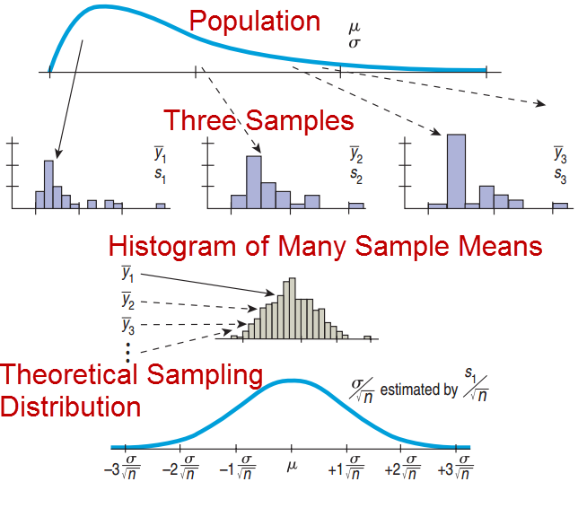
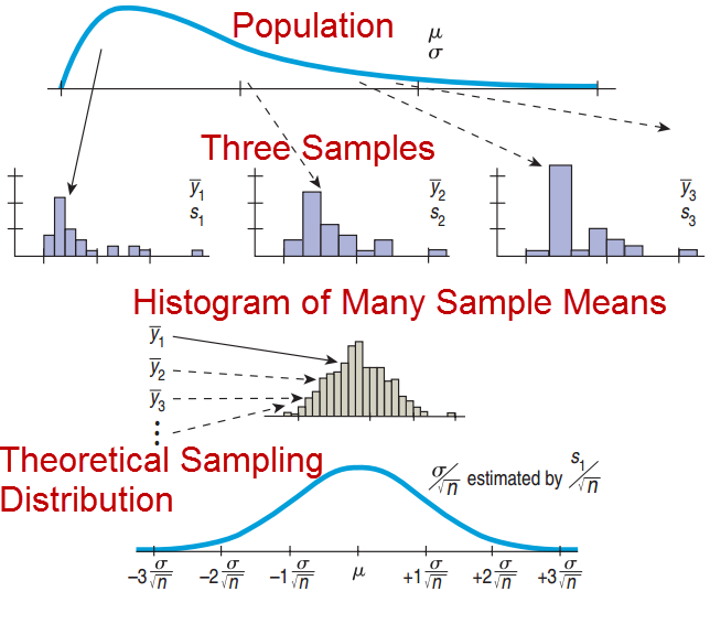
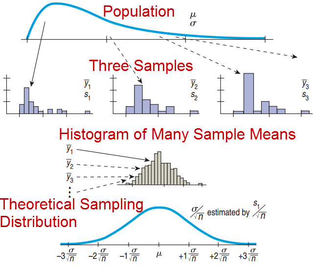
Sampling Distributions for Means (CLT)

$\sigma$ – the SD of the observations.

$\sigma^2$ – the variance of the observations.

s – the sample variance.

$\sigma/\sqrt{n}$ – the SD of sample means.

$\sigma^2/n$ – the variance of the sample means

Hand Washing Comparison

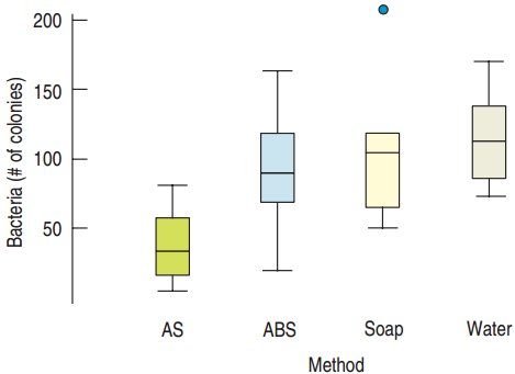
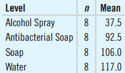
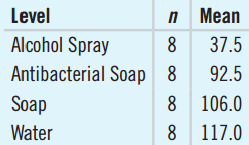
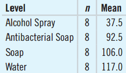
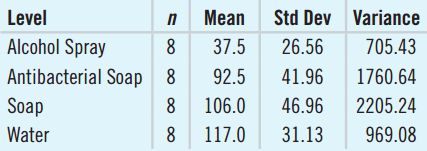
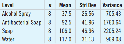
Is there a difference between washing hands with: water only, regular soap, antibacterial soap (ABS), and antibacterial spray (AS)?

Each tested with 8 replications
Treatments randomly assigned

Hand Washing

The means all differ.
Is this just natural variability? Is this happening by chance alone?
Null hypothesis: All the means are the same.
Alternative hypothesis: The means are not all the same.

26.1

Testing Whether the Means of Several Groups Are Equal

Comparing Many Means

H₀: All means are the same (= from same underlying population)
H_A: Not all the means are the same.

If all the same, then they should not vary too much. Maybe a little bit, because the samples are different (→ “sampling variability”)
Considering the means as data values, we measure the variance of this data.
If the means of the underlying population are different, the variance will be larger.

Variation within and between

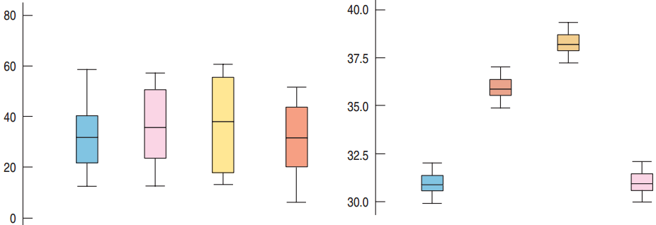
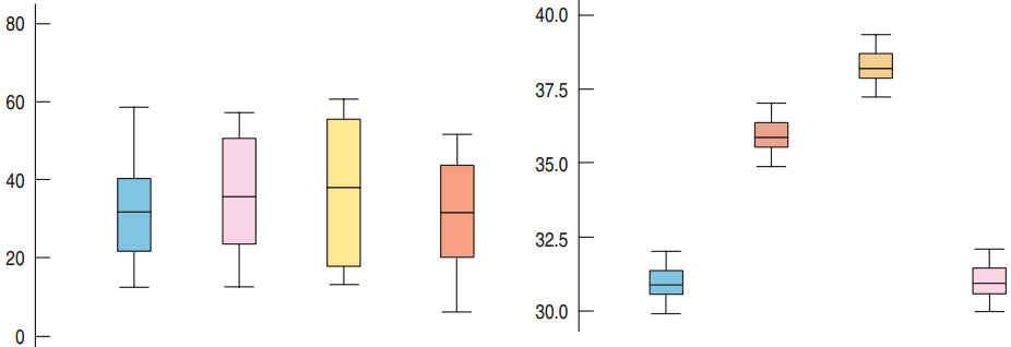
The means in the two examples are the same!
The variances are different

Comparing Means

The means in the two examples are the same!
The variances are different
Second case: the variation within is so small that the differences between stand out

Comparing Means

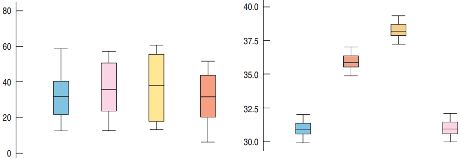
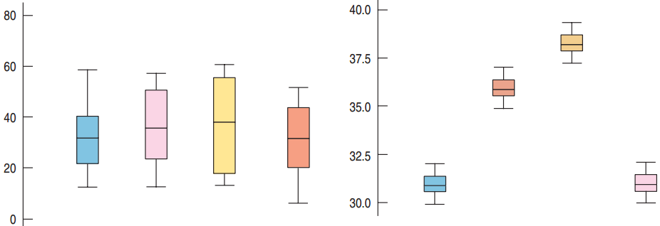
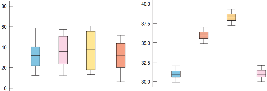
Note scales.
Left: Plausible that the means are equal. Large variance within each sample, not between samples.
Right: Means not equal. Small variance within samples, large variance between

Comparing Many Means: the F-test

Second case: the variation within is so small that the differences between stand out

This is the idea behind the F-test: we compare the variation within the groups with the variation between the groups
If Var Between > Var Within → we reject the null
If Var Between < Var Within → we fail to reject the null

Comparing Many Means: the variance BETWEEN

To compare two means: t-test on the difference.
To compare many means?
- If H₀ is true, there is a common mean.
- Look at the differences from this common mean.
- How do we do that?
- The variance of all the means does just that.
- This variance of the sample means is a measure of how much the sample means differ from each other.
- If H₀ is true, this variance should be small.

Washing Type All the Same?

H₀: $\mu_1 = \mu_2 = \mu_3 = \mu_4$
We will calculate the variance between these four sample means
We will use it to estimate $\sigma^2/n$, the variance of the sampling distribution of the means, and then $\sigma^2$, the variance of the observations.

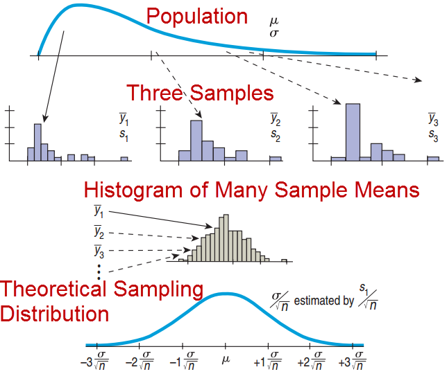
Sampling Distributions for Means (CLT)

$\sigma$ – the SD of the observations.

$\sigma^2$ – the variance of the observations.

s – the sample variance.

$\sigma/\sqrt{n}$ – the SD of means sampling dist.

$\sigma^2/n$ – the variance of means sampling dist.

Washing Type All the Same?

H₀: $\mu_1 = \mu_2 = \mu_3 = \mu_4$
We will calculate the variance between the means
We will use it to estimate $\sigma^2/n$, the variance of the sampling distribution of the means, and then $\sigma^2$, the variance of the observations.

1) First, by CLT: $\quad Var(\bar{y}) = \dfrac{\sigma^2}{n} = \dfrac{\sigma^2}{8}$
This is the variance of the sampling distribution of the means

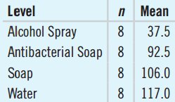
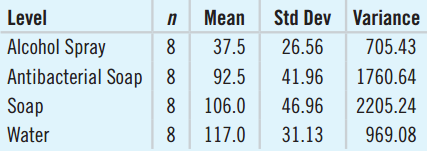
Variance of {37.5, 92.5, 106.0, 117.0} is 1245.08.

Washing Type All the Same?

H₀: $\mu_1 = \mu_2 = \mu_3 = \mu_4$
We will calculate the variance between the means
1) First, by CLT: $\quad Var(\bar{y}) = \dfrac{\sigma^2}{n} = \dfrac{\sigma^2}{8}$ ← variance of the SAMPLING DISTRIBUTION OF THE MEANS
Variance of {37.5, 92.5, 106.0, 117.0} is 1245.08.
2) $\quad \dfrac{\sigma^2}{8} = 1245.08 \rightarrow \sigma^2 = 9960.64$ ← I estimate the variance of OBSERVATIONS
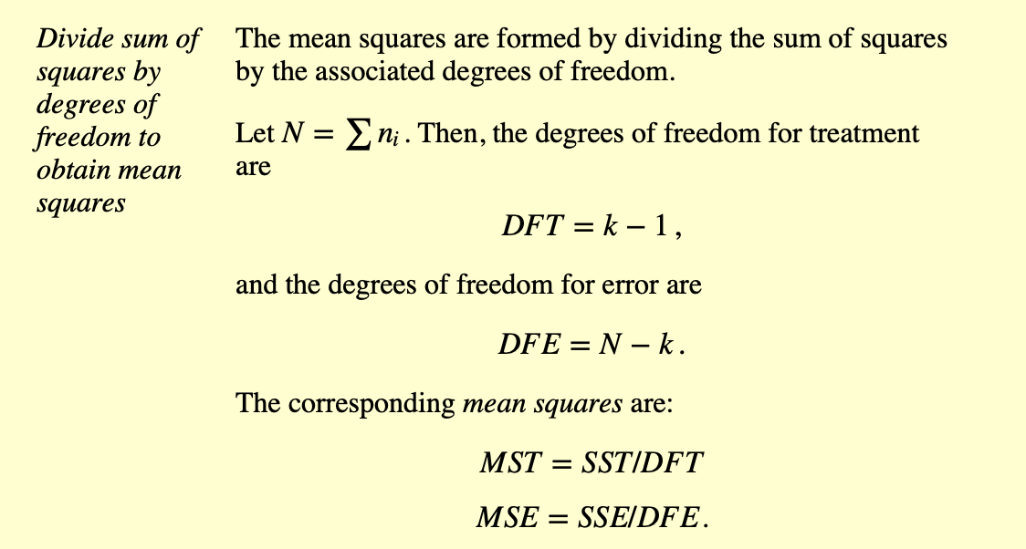
This estimate for $\sigma^2$ is called the Treatment Mean Square or MS_T,
Also: Between Mean Square, Regression Mean Square

Washing Type All the Same?

H₀: $\mu_1 = \mu_2 = \mu_3 = \mu_4$

\[\frac{\sigma^2}{8} = 1245.08 \rightarrow \sigma^2 = 9960.64\]

This estimate for $\sigma^2$ is called MS_T.

Estimates variance of OBSERVATIONS

MS_T depends on whether the means are equal or not

If the null were true, and the means were basically equal (belonging to the same distribution), then this variance is due only to sampling, only to the observations, so that MS_T perfectly estimates $\sigma^2$

Sampling Distributions for Means (CLT)

$\sigma$ – the SD of the observations.

$\sigma^2$ – the variance of the observations.

s – the sample variance.

$\sigma/\sqrt{n}$ – the SD of means sampling dist.

$\sigma^2/n$ – the variance of means sampling dist.

Washing Type All the Same?

H₀: $\mu_1 = \mu_2 = \mu_3 = \mu_4$

\[\frac{\sigma^2}{8} = 1245.08 \rightarrow \sigma^2 = 9960.64\]

This estimate for $\sigma^2$ is called MS_T

Variance of OBSERVATIONS

Depends on whether the means are equal or not
Means are closer → MS_T gets smaller
Means are farther apart → MS_T gets bigger → reject null
Is this very high compared to what we would expect?
To know, we need to compare it to another value.

Comparing Means

Note scales.
Left: Plausible that the means are equal. Large variance within each sample, not between samples.
Right: Means not equal. Small variance within samples, large variance between

The Variance WITHIN

There is another way to estimate the variance of observations $\sigma^2$: the variance within
Assume each washing method has the same sample variance (the variance of a specific sample)
Then we can pool them all together to get the pooled variance $s_p^2$.
Does not depend on whether means are equal or not
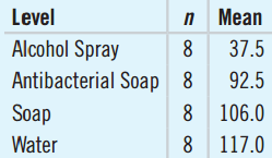
Since the sample sizes are all equal, we can average the four variances: $\ s_p^2 = 1410.10$.
Other names for $s_p^2$: Error Mean Square or MS_E, Within Mean Square. It estimates $\sigma^2$ directly.

Comparing MS_T and MS_E

MS_T (between)

Estimates $\sigma^2$ if H₀ is true and the means are equal
Should be larger than $\sigma^2$ if H₀ is false

MS_E (within)

Estimates $\sigma^2$ whether H₀ is true or not
If H₀ is true, both close to $\sigma^2$, so MS_T is close to MS_E

Comparing

If H₀ is true, MS_T / MS_E should be close to 1
If H₀ is false, MS_T / MS_E tends to be > 1
But how do we tell whether MS_T / MS_E is large enough?

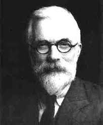
Sir Ronald Fisher Saves the Day!

How do we tell whether MS_T / MS_E is large enough to not be due just to random chance?
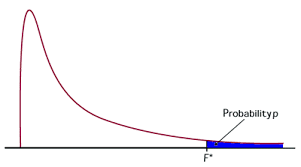
MS_T / MS_E follows the F-Distribution
- Numerator df: k – 1 (k = number of groups)
- Denominator df: k(n – 1)
- n = # observations in each group
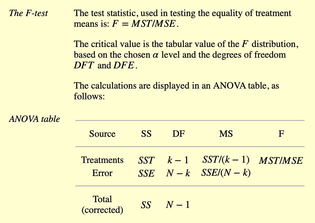
F = MS_T / MS_E is called the F-Statistic.

Analysis of Variance

The area to the right of the F-statistic represents the P-Value → probability I can get a more extreme value of F
If the P-value is small, we reject H₀ and conclude that there is evidence that the means are not all equal to each other.

Since both MS_T and MS_E come from looking at variances, we did an ANalysis Of Variance.
ANOVA

Back to Bacteria

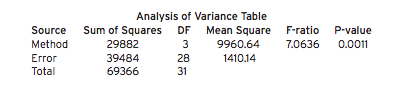
MS_T = 9960.64, MS_E = 1410.14

\[F = \frac{MS_T}{MS_E} = \frac{9960.64}{1410.14} \approx 7.06\]

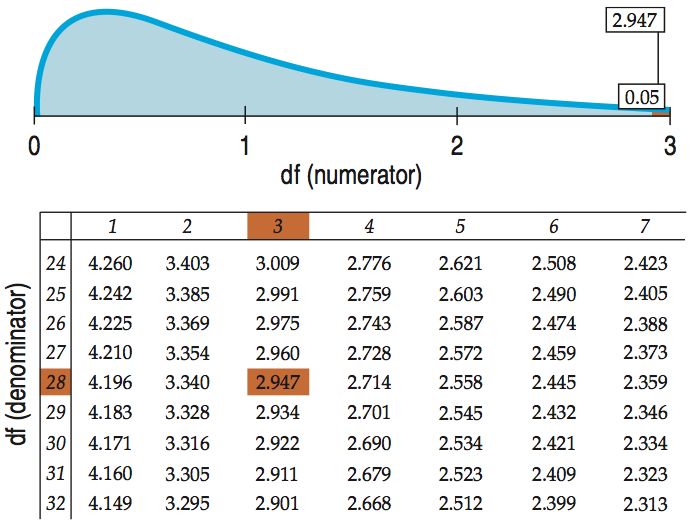
Num: df = 4 – 1 = 3, Den: df = 4(8 – 1) = 28.
Technology gives P-value for $F_{3,28}$ = 0.0011.

The F-Table

Conclusions About Hand Washing

If the means were all equal then only 11 in 10,000 experiments such as these would have MS_T / MS_E at least as large as 7.06.

We have strong evidence that the four different methods of hand washing are not equally effective at eliminating germs.

Residual Standard Deviation

To have the response variable’s units, we should work with the standard deviation instead of the variance:

\[s_p = \sqrt{MS_E} = \sqrt{\frac{\sum e^2}{N-k}}\]

$s_p$ is the residual standard deviation.
For the hand washing data: $s_p = \sqrt{1410.14} \approx 37.6$
This is a reasonable compromise standard deviation for all four groups.

26.2

The ANOVA Table

Contrast Baths

Contrast baths: To reduce hand swelling and stiffness in patients that had carpal tunnel release surgery, hands are alternately immersed in cold and hot water.

59 patients randomly assigned to one of:
- Contrast bath with no exercise
- Contrast bath with exercise
- Exercise but no contrast bath
Specify the subjects, sample size, experimental factor, treatment levels, response, null hypothesis, and research methods.

Contrast Baths

Subjects: Patients receiving carpal tunnel release surgery
Sample Size: 59
Factor: Contrast bath treatment
Levels: Contrast bath alone, Contrast with exercise, Exercise only.
Response: Change in hand volume
Null Hypothesis: Mean change in hand volume same for all three treatments
Methods: Single blind (patients but not the researchers aware of treatments)

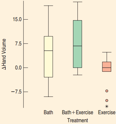
Bath Treatment

What does the boxplot tell us about the means for the three treatments?

. . .

Not much difference between the two contrast bath treatments.
The exercise only treatment may result in less swelling.

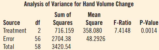
Hand Washing

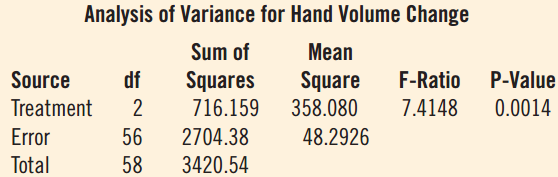
What does the ANOVA table say about the differences in the mean swelling for the three different types of contrast bath treatments?
- F = 7.4148 and the P-value is small.
- We can reject the null hypothesis that the mean change in hand volume is the same for all three treatments.

Hand Washing

26.3

Plot the Data

Assumptions and Conditions

To check the assumptions and conditions for ANOVA, always look at the side-by-side boxplots.
- Check for outliers within any group.
- Check for similar spreads.
- Look for skewness.
- Consider re-expressing.

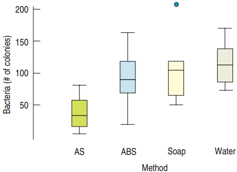
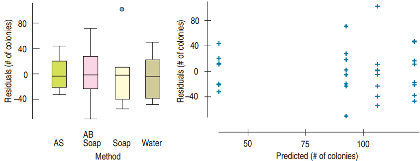
Checking Conditions for Hand Washing

IQR’s are about the same for all groups.
“The Plot Does Not Thicken.”
One outlier, not too extreme
$s_p$ = 37.6 reasonable for all four groups

Normal Population Assumption

Nearly Normal Condition

Must be satisfied for each group.
Use side-by-side boxplot to check for skewness and outliers.
Equal Variance Condition allows us to look at all the residuals together.
Use a histogram and Normal probability plot of all the data to check for Normality.

One Way ANOVA F-Test

H₀: $\mu_1 = \mu_2 = \dots = \mu_k$

\[F = \frac{MS_T}{MS_E}\]

MS_T is found FROM the variance BETWEEN means of the treatment groups.
MS_E is found by POOLING the variances WITHIN each of the treatment groups.
If F is large, reject H₀.

26.4

Comparing Means

What Next?

ANOVA:

P-value large → Nothing left to say
P-value small → Which means are large and which means are small?
We can perform a t-test to compare two of them.
We assumed the standard deviations are all equal.
Use $s_p$, for pooled standard deviations.
Use the Student’s t-model, df = N – k (N = total number of trials)

t-Test for Hand Washing

H₀: $\mu_W - \mu_{ABS} = 0$
H_A: $\mu_W - \mu_{ABS} \neq 0$
Diff. in observed means: 117.0 – 92.5 = 24.5.

\[SE(\mu_W - \mu_{ABS}) = s_p\sqrt{\frac{1}{n_W} + \frac{1}{n_{ABS}}} \approx 18.775\]

\[t = \frac{24.5}{18.775} \approx 1.31, \quad df = 32 - 4 = 28, \quad \text{P-value} = 0.2\]

We cannot discern a difference between washing with antibacterial soap and just using water.

Bonferroni Multiple Comparisons

If we wanted to do a t-test for each pair:
P(Type I Error) = 0.05 for each test.
Good chance at least one will have a Type I error.
Bonferroni devised a correction:
- Adjust $\alpha$ to $\alpha/J$ where J is the number of comparisons.
- 95% confidence (1 – 0.05) with 3 comparisons adjusts to (1 – 0.05/3) ≈ 0.98333.
- Use this adjusted value to find t**.

26.5

ANOVA on Observational Studies

The Trouble with Observational Studies

Difficult to verify equal variances.
May not have the same sample size for each treatment.
Without randomization, causation cannot be concluded even with a small P-value.
Cannot avoid lurking variables.
Since the subjects are not randomly assigned, the confidence interval may not represent the general population.

Who Watches More TV?

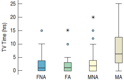
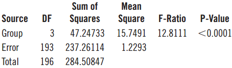
Four groups: male athletes (MA), male non-athletes (MNA), female athletes (FA), and female non-athletes (FNA) were surveyed. Do these four groups spend about the same amount of time watching TV?

Variables: Number of hours watching TV, the viewer’s gender and athlete status. Total of 197 randomly selected respondents.

Who Watches More TV?

Plot: Trouble! Each skewed, outliers (some extreme), category with highest center has a large spread.
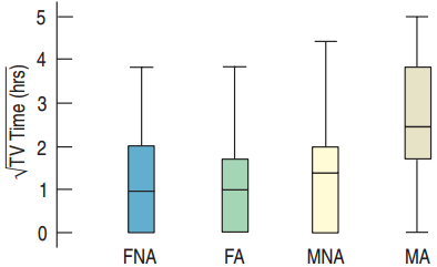
Re-express with a root.
- Randomization Condition: Students selected randomly.
- Similar Spread Condition: New boxplot much better.

Who Watches More TV?

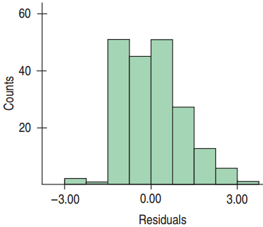
Nearly Normal Condition: Histogram of the residuals looks reasonably normal.
It is appropriate to use ANOVA.
Conclusion: The F-statistic is large and the corresponding P-value small. I conclude that the TV-watching behavior is not the same among these groups.

So Do Male Athletes Watch More TV?

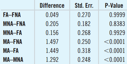
Bonferroni comparison of all pairs of groups.
Three significant differences:
- Male athletes watch more TV than both female athletes and non-athletes.
- Male athletes watch more than male non-athletes.
Does this generalize to all weeks and all colleges?
- The study was conducted during the NCAA men’s basketball tournament.

What Can Go Wrong?

Watch out for outliers.

Outliers affect most ANOVA statistics: mean, spread, F, P-value.
Increase P(Type II Error).

Watch out for changing variances.

ANOVA depends on independence, constant variance, and Normality.
If conditions on the residuals are violated, try re-expressing.

What Can Go Wrong?

Be wary of drawing conclusions about causality from observational studies.

Causality can only be concluded by ANOVA from randomized experiments.

Be wary of generalizing.

Don’t generalize if the data do not represent the general population.

Watch for multiple comparisons.

Use a multiple comparison method such as Bonferroni to test many pairs.

Chapter 27

Multifactor Analysis of Variance

27.1

A Two-Factor ANOVA Model

Two Factors at Once?!

Unlike experiments we have seen thus far, some studies have not one but two factors.

Example: study on accuracy throwing darts
Depends on which hand used and distance

Two Factors at Once?!

Two factors do not confuse things, but rather improve the experiment and analysis.
With two factors we have two hypotheses tests.
Each of those hypotheses asks whether the mean of the response variable is the same for each of the treatment levels.
Earlier, we considered ways to remove or avoid extra variation in designing experiments. A two-factor experiment does just that.

An ANOVA Model (cont)

Our null hypothesis on each factor is that the effects of that treatment are all zero (the means are equal)
The alternative hypotheses are that the treatment effects are not all equal (the means are different)
We want to compare the differences BETWEEN the treatment effects with the underlying variability WITHIN the treatment.

27.2

Assumptions and Conditions

Partial boxplots

Plot the Data …

Start by using side-by-side boxplots across levels of each factor.
Look for outliers and correct them or omit them if you can’t correct them.
The problem with looking at the boxplots is that the responses at each level of the factor contain all levels of the other factor.

Partial boxplots

Plot the Data …

A better alternative would be to make boxplots for each factor level after removing the effects of the other factor.
We could compute a one-way ANOVA on one factor and find the residuals. Then, make boxplots of those residuals for each level of the other factor. We might call this display a partial boxplot.

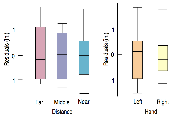
Dart-throwing study: partial boxplots

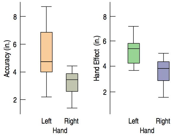
Boxplots of Accuracy by Hand (1) show the effect of changing Hand less clearly

Boxplots on the right (2) show the effects of Hand after the effect of Distance has been removed.

The effect of changing hands is much easier to see.

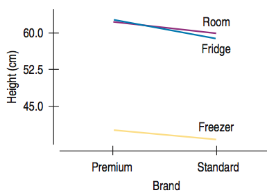
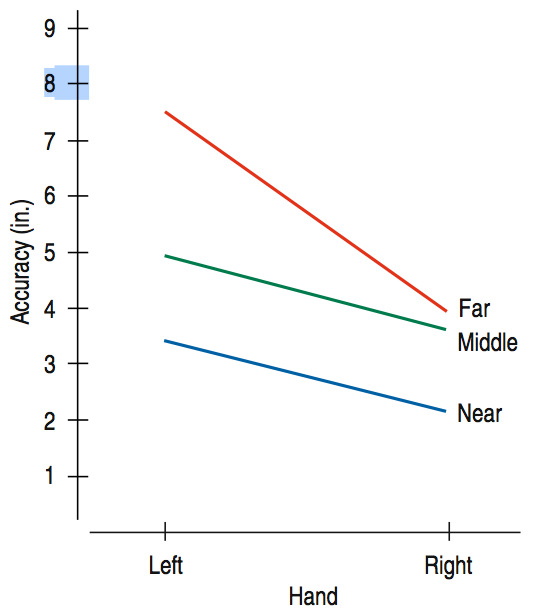
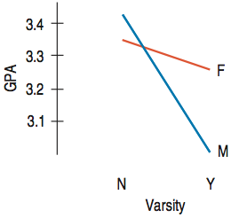
Interaction Plot

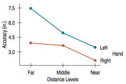
When the effects of one factor change for different levels of another factor, we say there is an interaction. To show the interaction, we use an interaction plot.

This plot shows the averages of the observations at each level of one factor broken up by the levels of the other factors.

Assumptions and Conditions

Independence Assumptions

An Independence Assumption for the two-factor model is the same as in a one-way ANOVA. Hence, the observations within each treatment group must be independent of each other. However, no test can verify that assumption.
Check the Randomization Condition. Were the data collected with suitable randomization? This is true for both surveys and experiments.

Assumptions and Conditions (cont)

Equal Variance Assumption

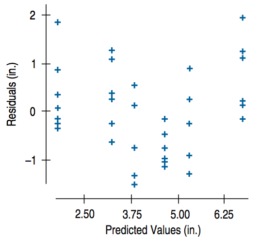
Like the one-way ANOVA, the two-factor ANOVA requires that the variances of all treatment groups be equal. We need to check for equal spread across all treatment groups.
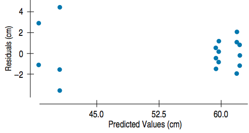
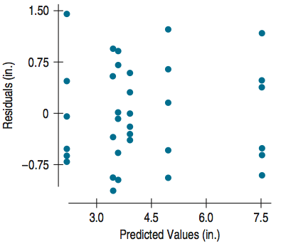
Look at the residuals plotted against the predicted values. If the plot thickens (to one side or the other), it’s a sign that the variance is changing systematically.
Consider re-expressing the response variable.

Assumptions and Conditions (cont)

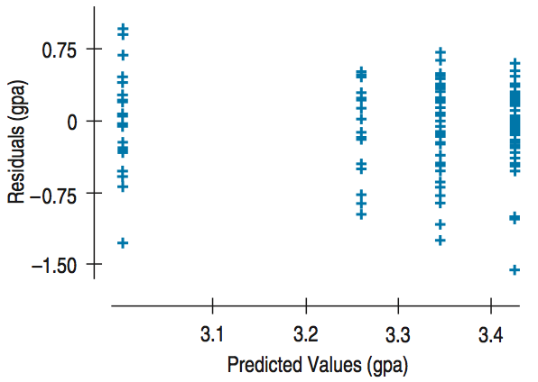
Scatterplot of residuals vs. predicted values from the two-way ANOVA model.
This figure doesn’t show changing variance, but it’s certainly not patternless. It shows a U-shaped pattern. This suggests the condition is violated.

Assumptions and Conditions (cont)

You can also plot the residuals grouped by each factor.

Boxplots of the residuals from the two-way ANOVA of the dart accuracy experiment show roughly equal variability when plotted for each factor.

Assumptions and Conditions (cont)

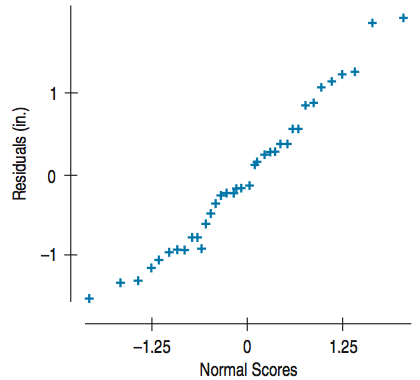
Normal Error Assumption

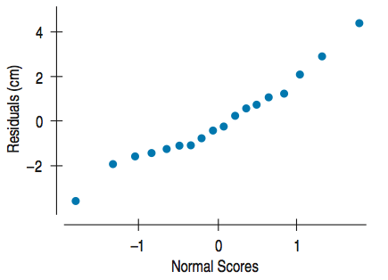
As with one-way ANOVA, the F-tests require that the underlying errors follow a Normal model. We’ll check a corresponding Nearly Normal Condition with a Normal probability plot or histogram of the residuals.

A Normal probability plot of the residuals from the two-way ANOVA model for dart accuracy seems reasonably straight.

Example: Two-Factor Analysis of Variance – Tennis balls’ bounce – Step-by-Step

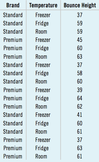
Perform a two-factor experiment on tennis balls Brand and Temperature, using two Brands of tennis balls and three levels of Temperature.
The subject bounced three balls under each of the six treatment conditions by first randomly selecting a Brand and for that ball, randomly selecting whether to leave it at room temperature or to put it in the refrigerator or the freezer. After 8 hours she dropped the balls from a height of 1 meter to a concrete floor, recording the Height of the bounce in centimeters.

Example: Two-Factor Analysis of Variance – Step-by-Step

This is a completely randomized replicated design in two factors.
The factor Brand has two levels: Premium and Standard.
The factor Temperature has three levels: Room, Fridge, and Freezer. The null hypotheses are that Brand has no effect and that Temperature has no effect.

Example: Two-Factor Analysis of Variance – Step-by-Step

State what we want to know and the null hypotheses we wish to test.

For two-factor ANOVA, the null hypotheses are that all the treatment groups have the same mean for each factor. The alternatives are that the means are not all equal.

Example: Two-Factor Analysis of Variance – Step-by-Step

Plan – Before Testing, Check Conditions.

Similar Variance Condition.

Example: Two-Factor Analysis of Variance – Step-by-Step

Nearly Normal Condition, Outlier Condition.

Example: Two-Factor Analysis of Variance – Step-by-Step

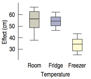
Plot – Examine the side-by-side partial boxplots of the data.

Temperature has an effect.
Can’t be sure about Brand from the plots.

Example: Two-Factor Analysis of Variance – Step-by-Step

Plan – Think about the assumptions and check the appropriate conditions.

Example: Two-Factor Analysis of Variance – Step-by-Step

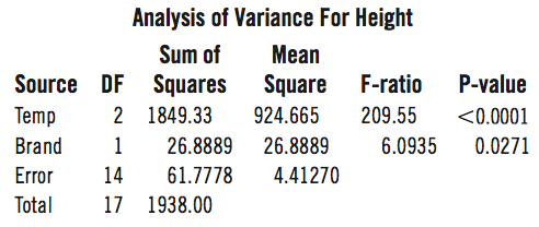
Plan – Show the ANOVA table.

Example: Two-Factor Analysis of Variance – Step-by-Step

Interpretation – Tell what the F-tests mean.

F-ratios this large would be very unlikely if the factors had no effect. I conclude that the means of the two Brand levels are not equal.

27.3

Interactions

Throwing darts: Interactions

Interaction plot of Accuracy by Hand and Distance. The effect of Distance appears to be greater for the left hand.

Example: Two-Factor ANOVA with Interaction – Step-By-Step

Earlier, we looked at how much TV four groups of students watched on average.
Let’s look at their grade point averages (GPAs).
We treated the four groups (male athletes, female athletes, male non-athletes, and female non-athletes) as four levels of the factor Group.
Now we recognize that there are really two factors: the factor Sex with levels male and female and the factor Varsity with levels yes and no. Let’s analyze the GPA data with a two-factor ANOVA.

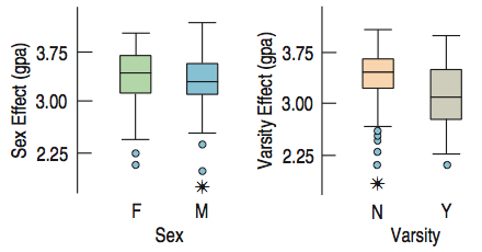
Example: Two-Factor ANOVA with Interaction – Step-By-Step

Plot – Examine the side-by-side partial boxplots of the data.

Example: Two-Factor ANOVA with Interaction – Step-By-Step

Similar Variance Condition:

no thickening, no pattern

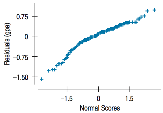
Nearly Normal Condition, Outlier Condition:

plot is reasonable

Example: Two-Factor ANOVA with Interaction – Step-By-Step

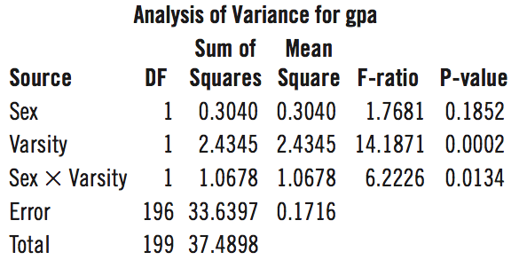
Plan – Show the ANOVA table.

Example: Two-Factor ANOVA with Interaction – Step-By-Step

What Can Go Wrong?

Always check for outliers.

Outliers can distort your conclusions.

Check for skewness.

If the underlying data distributions are skewed, consider a transformation to make them more symmetric.

Beware of unbalanced designs and designs with empty cells.

Empty cells and other more serious violations of balance require different methods and additional assumptions.

What Have We Learned?

We can extend the Analysis of Variance to designs with more than one factor.
Partial boxplots are a good way to examine the effect of each factor on the response.
Sometimes factors can interact with each other and we can add an interaction term to our model to account for the possible interaction.
We need to check the appropriate assumptions and conditions as we did for the simple ANOVA.

Careers

Where do we go from here

Roadmap

Human resources
Administrative positions
Higher Ed
Business/Data analyst
Psychologist → practice
Psychologist → research

Roadmap

Business/Data analyst
Psychologist → practice
Psychologist → research

Business and Data analyst

See: www.northeastern.edu/graduate/blog/data-analyst-vs-business-analyst/

Business analyst

data is a means to an end: make business decisions or evaluate businesses

Data analyst (aka statistician aka data scientist)

data is the end
other people ask questions
other people make decisions

Business and Data analyst

See: www.northeastern.edu/graduate/blog/data-analyst-vs-business-analyst/

Business analyst

data is a means to an end
background in business / psychology
general knowledge of programming

Data analyst

data is the end
background in STEM, master, PhD
specialized knowledge in programming, machine learning

Sport Analytics

Sport analytics

data is a means to an end
“Moneyball”

https://lacrossereference.com/2017/03/27/how-to-get-a-job-in-sports-analytics/

https://www.reddit.com/r/sportsanalytics/top/

Data scientists?

https://m.signalvnoise.com/data-scientists-mostly-just-do-arithmetic-and-thats-a-good-thing/

Data scientists?

https://m.signalvnoise.com/data-scientists-mostly-just-do-arithmetic-and-thats-a-good-thing/

“Knowing what matters is the real key to being an effective data scientist.”

“What you should probably do is make sure you understand how to do basic math, know how to write a basic SQL query, and understand how a business works and what it needs to succeed.”

Business and Data analyst

What do you need:

Quantitative skills
- Applied statistics
- Basic programming: spreadsheets, SQL, R and Python
Communication skills
- Public speaking (Toastmaster)
- Data visualization

Applied Statistics

Coursera: Improving your statistical inferences

https://www.coursera.org/learn/statistical-inferences

Learn statistics with R

https://learningstatisticswithr.com

Applied Statistics Books

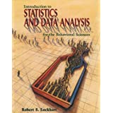
Introduction to Statistics and Data Analysis For the Behavioral Sciences

Model based book
More conceptual
PDF upload

Applied Statistics Books

Discovering Statistics Using R by Field, Miles, Field

Detailed, fun to read
A college course based on that book
https://www.usabart.nl/eval/

Applied Statistics Books

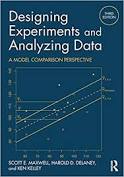
Designing Experiments and Analyzing Data: A Model Comparison Perspective, by Maxwell, Delaney, Kelley

Comprehensive, conceptually advanced but accessible
Ton of examples
Extra resources, code in R on book website

https://designingexperiments.com

Basic Programming

Datacamp (check out discounts)
Interested in Psychology? Focus on R (and then Python)
Interested in general programming? (focus on Python)
SQL courses on database management

Basic Programming

Codecademy
Khan Academy
Exercism
Dataquest
Teacup & Giraffes
- https://tinystats.github.io/teacups-giraffes-and-statistics/index.html
Online resources and communities
- https://makeawebsitehub.com/learn-to-code-for-free/
- https://www.reddit.com/r/learnprogramming/

Find what you like

Find what you like
Do one thing a day every day…
Once you get used to that, maybe do two things a day…

Practice psychology

Practice:
- Master in Counseling
- Master in Clinical Social Work
- PsyD
- PhD in Clinical Psychology
Research:
- Master in Experimental Psychology
- PhD in Clinical, Cognitive, Social Psychology or Neuroscience

Practice psychology

Practice:
- Master in Counseling
  - One or two years, can continue to PhD
  - Relatively easy to get in, but look for a good program
  - Tuition, a few scholarships?
- Master in Clinical Social Work
  - Two years, can continue to PhD
  - Relatively easy to get in, but look for a good program
  - Tuition, a few scholarships?
  - Very flexible

Practice psychology

Practice:
- PsyD
  - Five years, terminal degree
  - Relatively easy to get in
  - Tuition (expensive!) a few partial scholarships, or paid by employee
  - Look for a good program!
  - Excellent program here at Rutgers (GSAPP)
- PhD in Clinical Psychology
  - Five years, terminal degree
  - stipend; never pay for a PhD
  - Difficult to get in
  - Focused on research
  - Balance research/clinical practice may vary

Practice psychology

Research:
- Master in Experimental Psychology
  - One or two years
  - Relatively easy to get in
  - Tuition, a few partial or full scholarships
  - Example, master at Seton Hall
  - Stepping stone to a PhD
  - Find job as research associate in a lab (more common in neuroscience)
- PhD in (Clinical), Cognitive, Social Psychology or Neuroscience
  - Five years, terminal degree
  - Stipend; never pay for a PhD
  - Difficult to get in
  - Focused on research, some teaching
  - Transition from student to independent researcher
  - May be followed by a postdoc
  - After: Instructor, Professor, Research Associate
  - After: Business analyst, data analyst

What to do

Business analyst, data analyst:

Self-study (Datacamp, Dataquest, Coursera, online resources, Kaggle competitions etc.)
Take classes in basic programming, applied statistics, business
- Fall 2020: Programming for Behavioral Scientists
- 01:830:403 07373 Prof. Pernille Hemmer
Work on projects and showcase projects online
Internships as business analyst
Masters, Bootcamps etc.

What to do

Clinical and Research Psychology → Graduate School

Research experience
For the clinical route: clinical practice (class, volunteering, assistant etc.)
Letters of recommendation
Acquire quantitative skills: they will give you an edge in admissions
Take classes in basic programming, applied statistics, biostatistics
Work on projects and showcase projects online
Become a lab manager (difficult, based on networking)

Think about your goal and what you’d like to do

Learning quantitative skills can be boring/confusing/tiring/plain annoying
At times you’d like to smash the computer
Steep learning curve?
Codecademy, Khan Academy, Exercism FREE!
Datacamp, Dataquest about $30 a month (worth it if you like the platform – try free courses first)
Once you get into it, it’s fun!

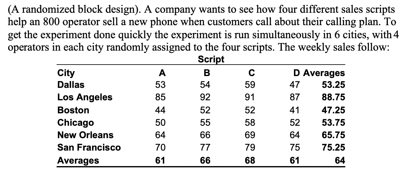
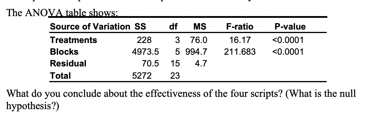
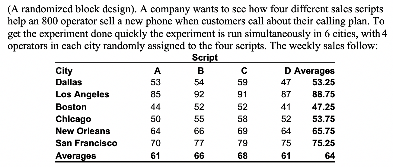
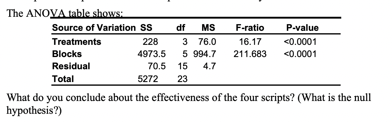
What are the factors?
From the table, what’s the MSE?
What’s the null hypothesis being tested by the F-ratio relative to treatments?
What’s the null hypothesis being tested by the F-ratio relative to blocks?
What are the alternative hypotheses?
What are your conclusions relative to the influence of treatments and blocks on sales effectiveness?

Quantitative Methods

Quantitative Methods

Announcements

Announcements: Final Exam

Announcements: Final Exam

Chapter 26

Analysis of Variance

The Sample Variance

*Sampling Distributions for Means (CLT)*

*Sampling Distributions for Means (CLT)*

Hand Washing Comparison

Hand Washing

26.1

Testing Whether the Means of Several Groups Are Equal

Comparing Many Means

Variation within and between

Comparing Means

Comparing Means

Comparing Many Means: the F-test

Comparing Many Means: the variance BETWEEN

Washing Type All the Same?

*Sampling Distributions for Means (CLT)*

Washing Type All the Same?

Washing Type All the Same?

Washing Type All the Same?

*Sampling Distributions for Means (CLT)*

Washing Type All the Same?

Comparing Means

The Variance WITHIN

Comparing MST and MSE

Sir Ronald Fisher Saves the Day!

Analysis of Variance

Back to Bacteria

The F-Table

Conclusions About Hand Washing

Residual Standard Deviation

26.2

The ANOVA Table

Contrast Baths

Contrast Baths

Bath Treatment

Hand Washing

Hand Washing

26.3

Plot the Data

Assumptions and Conditions

Checking Conditions for Hand Washing

Normal Population Assumption

One Way ANOVA F-Test

26.4

Comparing Means

What Next?

t-Test for Hand Washing

Bonferroni Multiple Comparisons

26.5

ANOVA on Observational Studies

The Trouble with Observational Studies

Who Watches More TV?

Who Watches More TV?

Who Watches More TV?

So Do Male Athletes Watch More TV?

What Can Go Wrong?

What Can Go Wrong?

Chapter 27

Multifactor Analysis of Variance

27.1

A Two-Factor ANOVA Model

Two Factors at Once?!

Two Factors at Once?!

An ANOVA Model (cont)

27.2

Assumptions and Conditions

Partial boxplots

Partial boxplots

Dart-throwing study: partial boxplots

Interaction Plot

Assumptions and Conditions

Assumptions and Conditions (cont)

Assumptions and Conditions (cont)

Assumptions and Conditions (cont)

Sampling Distributions for Means (CLT)

Sampling Distributions for Means (CLT)

Sampling Distributions for Means (CLT)

Sampling Distributions for Means (CLT)

Comparing MS_T and MS_E