Quantitative Methods

Lecture 20

Serena DeStefani

2020-08-11

Quantitative Methods

Serena DeStefani – Lecture 22 – 8/11/2020

How did we get here?

• Statistics is about variation, specifically in data
• Types of variables: continuous, categorical, ordinal
• How to represent variables
  • bar graphs
  • boxplots, histograms
• How to compare apples and oranges
  • by their variation (z scores)
  • are they varying together? correlation and regression

How did we get here?

• Statistics is about variation, specifically in data
• What am I interested in?
• A larger group, or population
• How to get data? Three ways

How do we get data?

1. Surveys
   • Impossible to survey the population
   • → representative sample (SRS) – randomized!
   • But exactly what does the population think?
   • What’s the population parameter?
2. Experiments
   • Randomized
   • Possible to infer causality
   • Is my result due to the treatment or is it due to chance?
3. Observational studies
   • Not possible to infer causality, or to extend findings
   • Sometimes necessary

A probability model

• Two questions:
  • What’s the population parameter?
  • Is my result likely?
• To answer these questions I need a probability model
• → The rules of probability
• Random variable: the Bernoulli trial (our building block)
• The geometric and binomial distribution
• The normal approximation to the binomial
• The sampling distribution
• The Central Limit Theorem

Summary

• How do we build a model for our data?
• Probability rules
• Random variable
• Random variable: the Bernoulli trial (our building block)
• Probability model (or probability distribution)
• There are many different distributions we can define and use, discrete or continuous.
• Examples:
  • Discrete: geometric or binomial
  • Continuous: normal, uniform, exponential
• Focus on binomial and normal distributions

The Binomial Model

• A Binomial probability model describes the number of successes in a specified number of trials.
• It takes two parameters to specify this model: the number of trials n and the probability of success p.

\[\text{Mean: } \mu = np\]

\[\text{Standard deviation: } \sigma = \sqrt{npq}\]

The Solution for Large Sample Sizes

• When the sample of our binomial model is too big, calculating probabilities becomes too complicated → use a normal model to approximate it.
• First we calculate mean and SD according to the binomial model.
• Then we use a normal model with the same mean and standard deviation as a very good approximation.
• If we have a normal model, we can use z-scores to calculate probabilities.
• For the approximation to work, we need at least 10 successes and 10 failures.

Sampling About Climate Change

According to a Gallup poll of 1022 Americans, 57% believe that climate change is due to human activity.

• If many surveys were done of 1022 Americans, we could calculate the sample proportion for each.
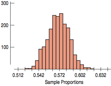
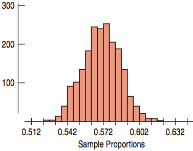
• The histogram shows the distribution of a simulation of 2000 sample proportions.
• The distribution of all possible sample proportions from samples with the same sample size is called the sampling distribution.

Sampling Distributions for Proportions

Sampling Distribution for Proportions

• Symmetric
• Unimodal
• Centered at p
• The sampling distribution follows the Normal model.

What does the sampling distribution tell us?

• The sampling distribution allows us to make statements about where we think the corresponding population parameter is and how precise these statements are likely to be.

From One Sample to Many Samples

Distribution of One Sample

• Variable was the answer to the survey question or the result of an experiment.
• Proportion is a fixed value that comes from the one sample.

Sampling Distribution

• Variable is the proportion that comes from the entire sample.
• Many proportions that differ from one to another, each coming from a different sample.

Mean and Standard Deviation

Sampling Distribution for Proportions

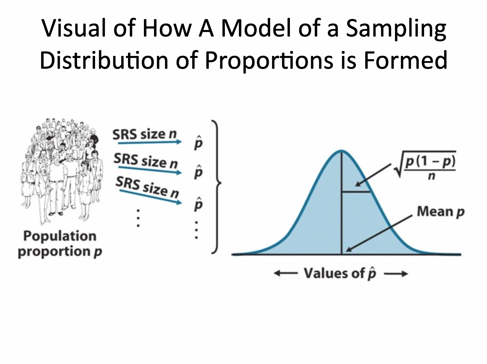
• \(\text{Mean} = p\)
• \(\sigma(\hat{p}) = \dfrac{\sqrt{npq}}{n} = \sqrt{\dfrac{pq}{n}}\)
• \(N\left(p, \sqrt{\dfrac{pq}{n}}\right)\)

This p is a parameter!

Instead \(\hat{p}\) is a statistic!

The Normal Model for Climate Change

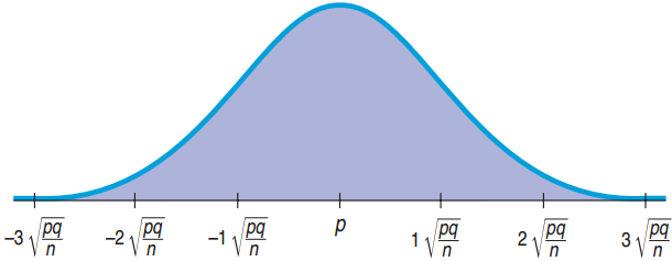
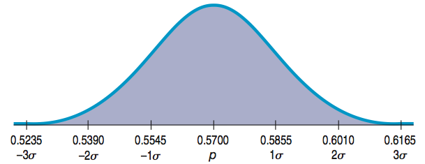
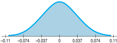
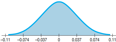
Population: p = 0.57, n = 1022. Sampling Distribution:

• Mean = 0.57
• Standard deviation \(= SD(\hat{p}) = \sqrt{\dfrac{(0.57)(0.43)}{1022}} \approx 0.0155\)

Standard Error

The sample-to-sample standard deviation is called the standard error or sampling variability.

• The standard error is not a “real” error, since no error has been made.

The problem is, we don’t know the population parameter.

Sampling Distribution

• Model a proportion with a binomial (yes/no)
• Large n: approximate with normal

• What about the mean?
• Can we build a sampling distribution for the mean?
• What will be its shape?

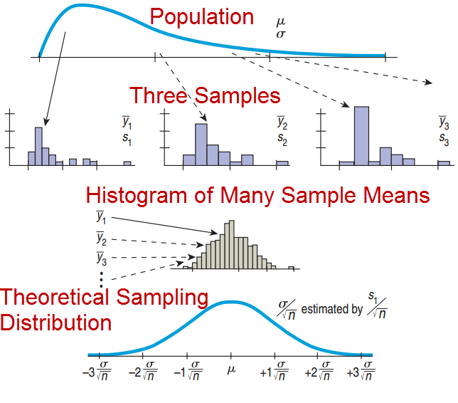
The Central Limit Theorem (CLT): sampling distribution for the mean

The mean of a random sample is a random variable whose sampling distribution can be approximated by a Normal model. The larger the sample, the better the approximation will be.

Population Distribution and Sampling Distribution of the Means

Population Distribution

• Normal
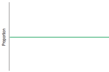
• Uniform
• Bimodal
• Skewed

Sampling Distribution for the Means

• → Normal (any sample size)
• → Normal (large sample size)
• → Normal (larger sample size)
• → Normal (larger sample size)

The Sampling Distribution Model for a Mean

When a random sample is drawn from a population with mean \(\mu\) and standard deviation \(\sigma\), the sampling distribution has:

• Mean: \(\mu\)
• Standard Deviation: \(\dfrac{\sigma}{\sqrt{n}}\)
• For large sample size, the distribution is approximately normal regardless of the population the random sample comes from.
• The larger the sample size, the closer to Normal.

Our questions:

• What’s the population parameter?
  • → Confidence Intervals
• Is my result likely?
  • → Hypothesis testing

Where are we going?

• Confidence intervals
• Hypothesis testing for proportions
• Hypothesis testing for means
• What if I have counts? → Chi-square tests
• What if I want to test an association? → hypothesis testing for regression
• What if I have more than two groups? → Analysis of Variance (ANOVA)

Confidence intervals for proportions

Capturing a Proportion

• The confidence interval may or may not contain the true population proportion.
• Consider repeating the study over and over again, each time with the same sample size.
  • Each time we would get a different \(\hat{p}\).
  • From each \(\hat{p}\), a different confidence interval could be computed.
  • About 95% of these confidence intervals will capture the true proportion.
  • 5% will not.

Simulating Confidence Intervals

Confidence Intervals

There are a huge number of confidence intervals that could be drawn.

• In theory, all the confidence intervals could be listed.
• 95% will “work” (capture the true proportion).
• 5% will not capture the true proportion.

What about our confidence interval (0.234, 0.382)?

• We will never know whether it captures the population proportion.
• “Statistics Means Never Having to Say You Are Certain”

Margin of Error

• Confidence interval for a population proportion (95%):

\[\hat{p} \pm 2SE(\hat{p})\]

• The distance, \(2SE(\hat{p})\), from \(\hat{p}\) is called the margin of error.
• Confidence intervals also work for means, regression slopes, and others. In general, the confidence interval has the form

\[\text{Estimate} \pm ME\]

Critical Values

• For a 95% confidence interval, the margin of error was 2SE.
  • The 2 comes from the normal curve.
  • 95% of the area is within about 2SE from the mean.
• In general the number of SE is called the critical value. Since we use the normal distribution here we denote it z*
• To be more precise, z* for 95%CI is 1.96

Finding the Critical Value

Find the critical value corresponding to 90% confidence.

• 90% inside gives 10% outside.
• 2 tails outside with 10% means 1 tail with 5% or 0.05.
• The critical value is about z* = 1.645.

Finding the Margin of Error (Take 2)

Yale/George Mason Poll: 1010 US adults, 40% think scientists disagree about global warming. At 95% confidence ME = 3%.

• Find the margin of error at 90% confidence.

Finding the Margin of Error (Take 2)

Yale/George Mason Poll: 1010 US adults, 40% think scientists disagree about global warming. At 95% confidence ME = 3%.

• Find the margin of error at 90% confidence.

\[SE(\hat{p}) = \sqrt{\frac{(0.4)(0.6)}{1010}} \approx 0.0154\]

• For 90%, z* ≈ 1.645: ME = (1.645)(0.0154) = 0.025.
• This gives a smaller margin of error which is good.
• Drawback: lower level of confidence which is bad

One-Proportion z-Interval

• First check for randomization, independence, 10%, and conditions on sample size.
• Confidence level C, sample size n, proportion \(\hat{p}\).
• Confidence interval: \(\hat{p} \pm z^{*}SE(\hat{p})\)

\[SE(\hat{p}) = \sqrt{\frac{(\hat{p})(\hat{q})}{n}}\]

• z*: the critical value that specifies the number of SE’s needed for C% of random samples to yield confidence intervals that capture the population proportion.

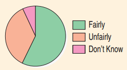
Do You Believe the Death Penalty is Applied Fairly?

• Sample size: 510
• Answers:
  • 58% “Fairly”
  • 36% “Unfairly”
  • 7% “Don’t Know”
• Construct a confidence interval for the population proportion that would reply “Fairly.”

Do You Believe the Death Penalty is Applied Fairly?

• Plan: Find a 95% confidence interval for the population proportion.
• Model:
  • Randomization: Randomly selected by Gallup Poll
  • 10% Condition: Population is all Americans
  • Success/Failure Condition
    • (510)(0.58) = 296 ≥ 10, (510)(0.42) = 214 ≥ 10
  • Use the Normal Model to find a one-proportion z-interval.

Do You Believe the Death Penalty is Applied Fairly?

• Mechanics: n = 510, \(\hat{p} = 0.58\)

Do You Believe the Death Penalty is Applied Fairly?

• Mechanics: n = 510, \(\hat{p} = 0.58\)

\[SE(\hat{p}) = \sqrt{\frac{(0.58)(0.42)}{510}} \approx 0.022\]

• z* ≈ 1.96
• ME ≈ (1.96)(0.022) ≈ 0.043
• The 95% Confidence Interval is: 0.58 ± 0.043 or (0.537, 0.623)

Do You Believe the Death Penalty is Applied Fairly?

• Conclusion: I am 95% confident that between 53.7% and 62.3% of all US adults think that the death penalty is applied fairly.

Inference about proportions

Cracking Rate < 20%?

General cracking rate: 20%

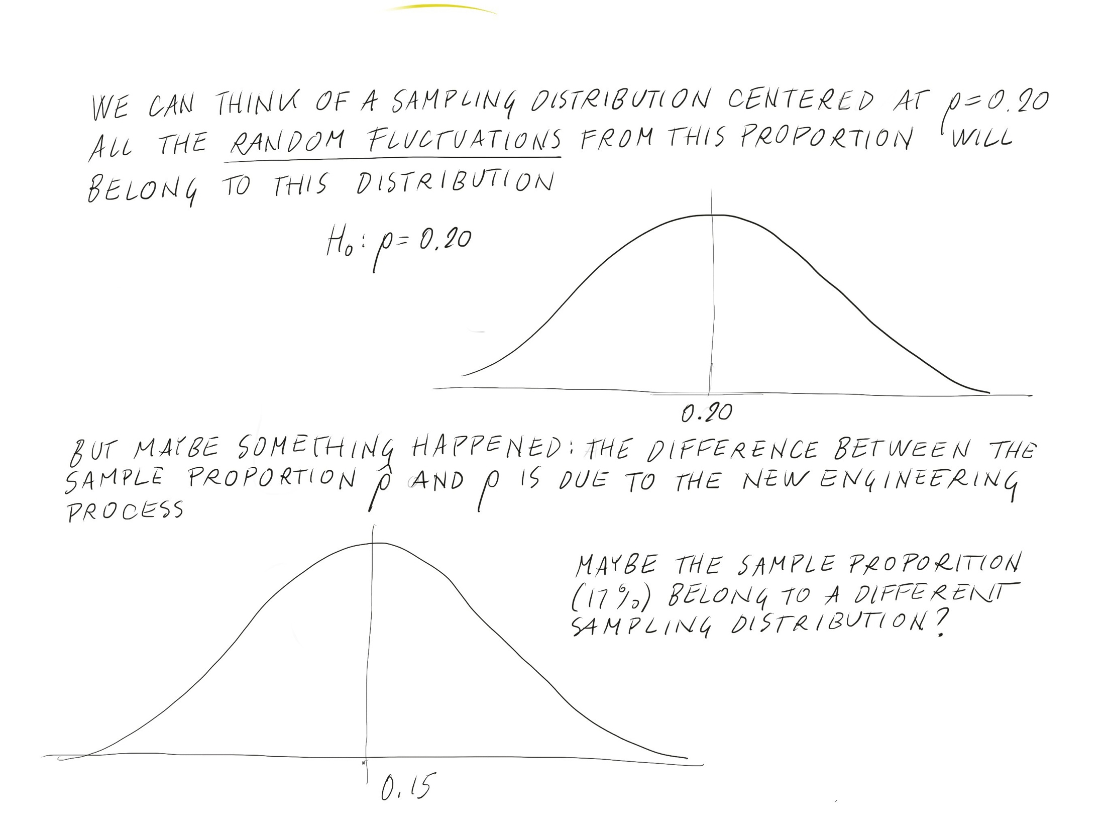
After a new engineering process, the cracking rate of 400 casts fell to 17%.

Is this due to the new engineering or just random chance?

• Null Hypothesis: Nothing has changed
  • H₀: parameter = hypothesized value
  • H₀: p = 0.20
• Alternative Hypothesis:
  • H_A: p < 0.20

How Small to Convince Us?

• Had the new cracking rate been 1%, it would clearly indicate a change from 20%.
  • Extremely unlikely that this could happen just by random chance
• Had the new cracking rate been 19.8%, we would be skeptical.
  • Not so unlikely to be just random chance
• How about 17%?
  • How likely is it that a random sample would have a cracking rate 17% or less?

Checking Conditions and Finding the Standard Error

Checking Conditions: n = 400, p = 0.20

• np = (400)(0.20) = 80 ≥ 10
• nq = (400)(0.80) = 320 ≥ 10
• Independence plausible
• The Normal model applies.

Find the standard deviation of the model.

\[SD(\hat{p}) = \sqrt{\frac{pq}{n}} = \sqrt{\frac{(0.20)(0.80)}{400}} = 0.02\]

• Note: Use p and not \(\hat{p}\) to find standard deviation.

Using the Normal Model

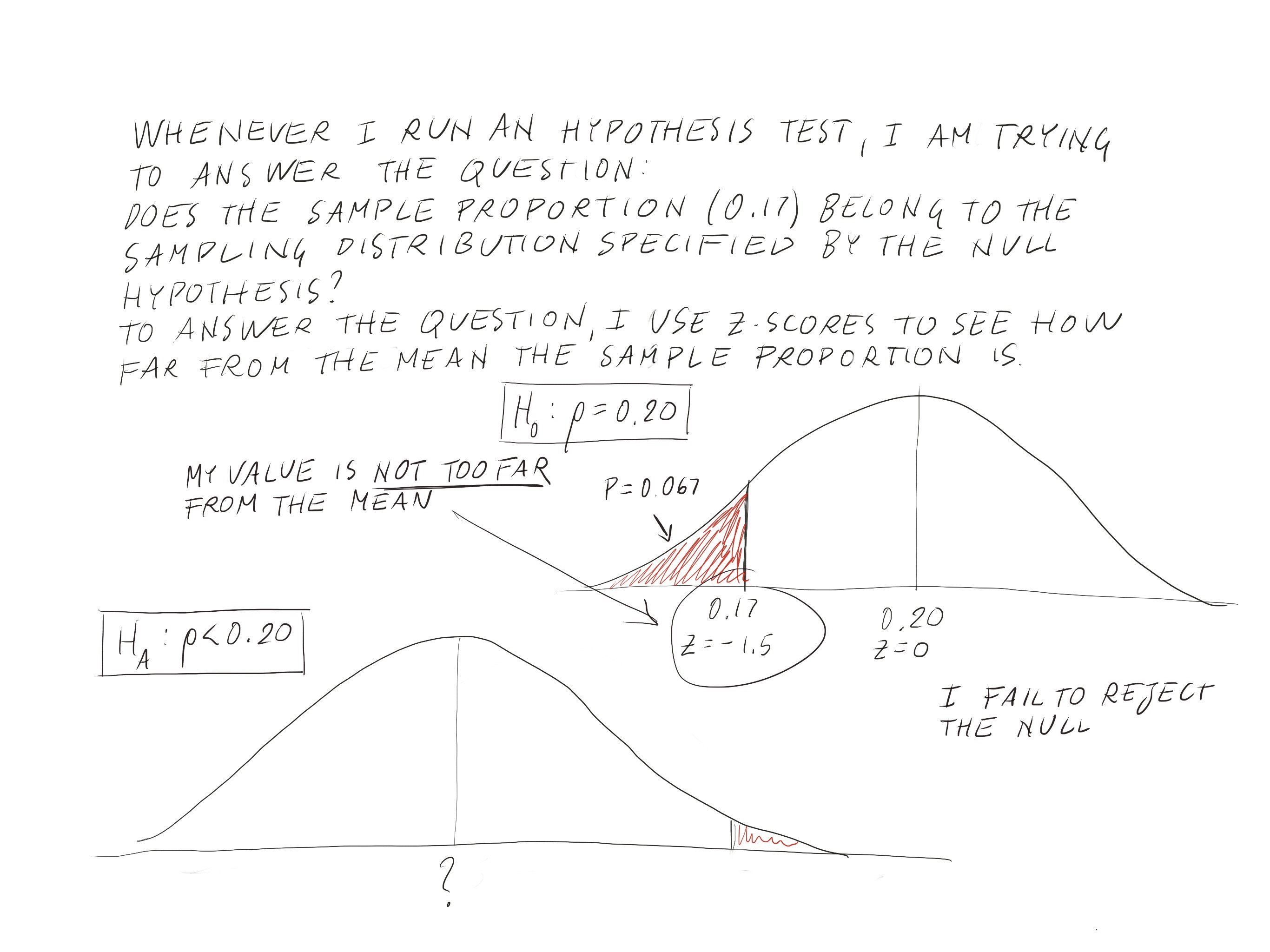
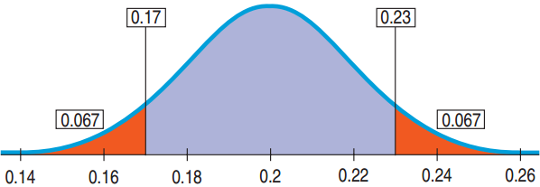
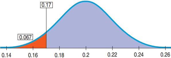
p = 0.20, \(\hat{p}\) = 0.17, \(SD(\hat{p})\) = 0.02

Using the Normal Model

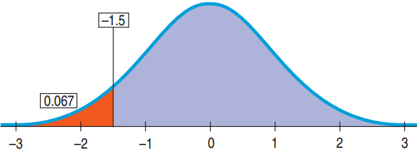
p = 0.20, \(\hat{p}\) = 0.17, \(SD(\hat{p})\) = 0.02

\[z = \frac{0.17 - 0.20}{0.02} = -1.5\]

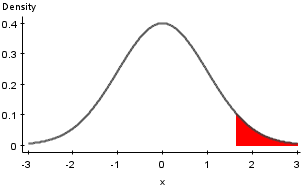
\[P(z < -1.5) \approx 0.067\]

• If the null hypothesis is true that the cracking rate is still equal to 20%, then the probability of observing a cracking rate of 17% in a random sample of 400 is 6.7%.

When the P-Value is Not Small

Wrong

• Accept H₀.
• We have proven H₀.

Right

• Fail to reject H₀
• There is insufficient evidence to reject H₀.
• H₀ may or may not be true.

Example: H₀: All swans are white.

• If we sample 100 swans that are all white, there could still be a black swan.

Step 1: State the Hypotheses

H₀:

• H₀ usually states that there’s nothing different.
• H₀: parameter = hypothesized value
• Note the parameter describes the population not the sample.
• H₀ is called the null hypothesis.

H_A:

• H_A is a statement that something has changed, gotten bigger or smaller or just different
• H_A is called the alternative hypothesis.

Hypotheses About the DMV

The DMV claims 80% of all drivers pass the driving test. In a survey of 90 teens, only 61 passed.

• Is there evidence that teen pass rates are below 80%?
  • H₀: p = 0.80
  • H_A: p < 0.80

1-Proportion z-Test

Conditions

• Same as a 1-Proportion z-Interval

Null Hypothesis

• H₀: p = p₀

Test Statistic:

\[z = \frac{\hat{p} - p_0}{SD(\hat{p})} \qquad SD(\hat{p}) = \sqrt{\frac{p_0 q_0}{n}}\]

DMV Study: Mechanics

Claim: 80% pass. 61 of 90 teens tested passed.

• n = 90, x = 61, p₀ = 0.80,

DMV Study: Mechanics

Claim: 80% pass. 61 of 90 teens tested passed.

• Find P-value.
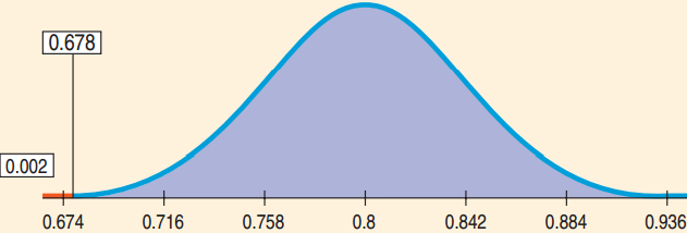
• n = 90, x = 61, p₀ = 0.80, \(\hat{p} = \dfrac{61}{90} \approx 0.678\)

\[SD(\hat{p}) = \sqrt{\frac{p_0 q_0}{n}} \approx \sqrt{\frac{(0.80)(0.20)}{90}} \approx 0.042\]

\[z = \frac{0.678 - 0.80}{0.042} \approx -2.90\]

\[\text{P-value} = P(z < -2.90) \approx 0.002\]

DMV Study: Conclusion

Is the teen pass rate less than 80%? P-value = 0.002

• What can be concluded? What does the P-value mean?
  • P-value = 0.002 is very small → Reject H₀
  • The survey data provide strong evidence that the pass rate for teens is less than 80%.
  • This should not be the end of the conversation.
  • The next step would be to see if the pass rate is low enough to take further action.

Two-Sided Alternative

For the new process the engineer may be interested in whether there has been a change in the cracking rate not just a decrease.

• H₀: p = 0.20
• H_A: p ≠ 0.20

• An alternative hypothesis where we are interested in deviation on either side is called a two-sided alternative.
• The P-value is the probability of deviating from either direction from the null hypothesis.

One-Sided Alternative

The engineer may be interested in whether there has been a decrease in the cracking rate.

• H₀: p = 0.20
• H_A: p < 0.20

• An alternative hypothesis where we are interested in deviation on only one side is called a one-sided alternative.
• The P-value for a one-sided alternative is always half the P-value for the two-sided alternative.
• The P-value for a two-sided alternative is always double the P-value for the one-sided alternative.

Inference about means

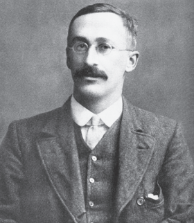
Gosset at Guinness

At Guinness, Gosset experimented with beer.

• The Normal Model was not right for small samples.
• Right model still bell shaped, but details differed, depending on n
• Came up with the “Student’s t Distribution” as the correct model

Degrees of Freedom

• For every sample size n there is a different Student’s t distribution.
• Degrees of freedom: df = n – 1.
• Similar to the “n – 1” in the formula for sample standard deviation
• It is the number of independent quantities left after we’ve estimated the parameters.

Confidence Interval for Means

Sampling Distribution Model for Means

• With certain conditions (seen later), the standardized sample mean follows the Student’s t model with n – 1 degrees of freedom.

\[t = \frac{\bar{y} - \mu}{SE(\bar{y})}\]

• We estimate the standard deviation with

\[SE(\bar{y}) = \frac{s}{\sqrt{n}}\]

One Sample t-Interval for the Mean

• When the assumptions are met (seen later), the confidence interval for the mean is

\[\bar{y} \pm t^{*}_{n-1} \times SE(\bar{y})\]

• The critical value \(t^{*}_{n-1}\) depends on the confidence level, C, and the degrees of freedom n – 1.

Thoughts about z and t

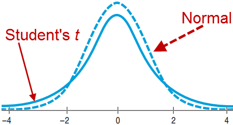
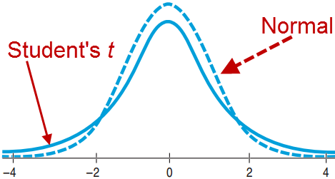
• The Student’s t distribution:
  • Is unimodal.
  • Is symmetric about its mean.
  • Has higher tails than Normal.
  • Is very close to Normal for large df.
  • Is needed because we are using s as an estimate for \(\sigma\).

• If you happen to know \(\sigma\), which almost never happens, use the Normal model and not Student’s t.

One-Sample t-Test for the Mean

• Assumptions are the same.
• H₀: \(\mu = \mu_0\)

\[t_{n-1} = \frac{\bar{y} - \mu_0}{SE(\bar{y})}\]

• Standard Error of \(\bar{y}\): \(SE(\bar{y}) = \dfrac{\sigma}{\sqrt{n}}\)
• When the conditions are met and H₀ is true, the statistic follows the Student’s t Model.
• Use this model to find the P-value.

Are the Salmon Unsafe?

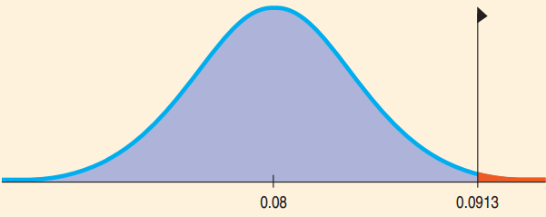
EPA recommended mirex screening is 0.08 ppm.

• Are farmed salmon contaminated beyond the permitted EPA level?
• Recap: Sampled 150 salmon. Mean 0.0913 ppm, Standard Deviation 0.0495 ppm.
• H₀: \(\mu = 0.08\)
• H_A: \(\mu > 0.08\)

Are the Salmon Unsafe?

One-Sample t-Test for the Mean

• n = 150, df = 149, \(\bar{y}\) = 0.0913, s = 0.0495

Are the Salmon Unsafe?

One-Sample t-Test for the Mean

• n = 150, df = 149, \(\bar{y}\) = 0.0913, s = 0.0495

\[SE(\bar{y}) = \frac{0.0495}{\sqrt{150}} \approx 0.0040, \quad t_{149} = \frac{0.0913 - 0.08}{0.0040} = 2.825\]

\[P(t_{149} > 2.825) = 0.0027\]

• or P < 0.005 using the t-table
• Since the P-value is so low, reject H₀ and conclude that the population mean mirex level does exceed the EPA screening value.

Intervals and Tests

Confidence Intervals

• Start with data and find plausible values for the parameter.
• Always 2-sided

Hypothesis Tests

• Start with a proposed parameter value and then use the data to see if that value is not plausible.

The Special Case with Proportions!

Confidence Intervals

• Use \(\hat{p}\) to calculate \(SE(\hat{p})\).

Hypothesis Tests

• Use p to calculate SD(p).

Considerations on \(\alpha\) and type I & II errors

Choosing an \(\alpha\)

• \(\alpha\) = 0.05 is most common.
  • (1 in 20 chances is pretty rare)
• Other levels of significance commonly used:
  • 0.001, 0.01, 0.1
• Are the air bags safe?
  • Low \(\alpha\) such as 0.001.
• Do students like pepperoni or sausage?
  • High \(\alpha\) such as 0.1.

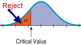
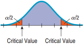
Critical Values: An Alternative to P-Values.

• For a hypothesis test look at the z-axis (or t-axis) to decide on whether to reject H₀.
• Find the value of z (or t) that corresponds to \(\alpha\).
• 2-tails: use \(\alpha/2\)

Confidence Intervals and Hypothesis Tests

• A confidence interval contains all plausible values.
• Two Tailed Test: Any hypothesized value outside will be rejected. \(\alpha\) = 100 – C.
  • C = 95% → \(\alpha\) = 5%
• One Sided Test: \(\alpha\) = ½ (100 – C)
  • C = 95% → \(\alpha\) = ½(100 – 95) = 2.5%

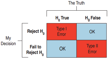
Type I and II Errors

Type I Error

• Reject H₀ when H₀ is true.

Type II Error

• Fail to reject H₀ when H₀ is false.

Medicine: Such as an AIDS test

• Type I Error → False positive: Healthy person is diagnosed with the disease.
• Type II Error → False negative: Infected person is diagnosed as disease free.

Type I and II Errors

Jury Decisions

• Type I: Found guilty when the defendant is innocent. Put an innocent person in jail.
• Type II: Not enough evidence to convict, but was guilty. A murderer goes free.

Inference for difference between proportions

Review: Two-Proportion z-Interval

If the conditions are met, the confidence interval for p₁ – p₂ is

\[\left(\hat{p}_1 - \hat{p}_2\right) \pm z^{*} \times SE\left(\hat{p}_1 - \hat{p}_2\right)\]

\[SE\left(\hat{p}_1 - \hat{p}_2\right) = \sqrt{\frac{\hat{p}_1\hat{q}_1}{n_1} + \frac{\hat{p}_2\hat{q}_2}{n_2}}\]

• z* is the critical value that corresponds to the confidence level C.

Review: Hypothesis Test - Pooling the Proportions

• H₀ comparing two proportions: proportions are equal.
• To do a hypothesis test, we assume that the proportions are equal
• We should have only one value for proportion
• Total successes: 205 + 235 = 440
• Total trials: 293 + 469 = 762
• Pooled Proportion:

\[\hat{p}_{pooled} = \frac{Success_1 + Success_2}{n_1 + n_2} = \frac{440}{762} \approx 0.5774\]

Two-Proportion z-Test

• Conditions same as 2-proportion CI.
• H₀: p₁ – p₂ = 0

\[\hat{p}_{pooled} = \frac{Success_1 + Success_2}{n_1 + n_2}\]

\[SE_{pooled}\left(\hat{p}_1 - \hat{p}_2\right) = \sqrt{\frac{\hat{p}_{pooled}\,\hat{q}_{pooled}}{n_1} + \frac{\hat{p}_{pooled}\,\hat{q}_{pooled}}{n_2}}\]

\[z = \frac{\hat{p}_1 - \hat{p}_2 - 0}{SE_{pooled}\left(\hat{p}_1 - \hat{p}_2\right)}\]

• The statistic follows the Normal model.

Pre-Sleep Internet Rates Differ?

• Plan: Random sample of adults:
• 293 Gen Y (19-29 years old)
• 469 Gen X (30-45 years old)
• Percentage reporting using internet before sleep
• Hypotheses:
  • H₀: p_GenY – p_GenX = 0
  • H_A: p_GenY – p_GenX ≠ 0
• Model
  • Randomization Condition: Randomly selected and stratified by sex.

Pre-Sleep Internet Rates Differ?

• Model (Continued)
  • 10% Condition: Samples less than 10% of all Gen X and Gen Y.
  • Independent Groups Assumption: The samples were selected at random so independent.
  • Success/Failure Condition: Observed numbers of successes and failures for both groups ≥ 10.
• The conditions are all met. Use the Normal model and perform a two-proportion z-test.

Pre-Sleep Internet Rates Differ?

• Mechanics:

\[n_{GenY} = 293, \; y_{GenY} = 205, \; \hat{p}_{GenY} = 0.700\]

\[n_{GenX} = 469, \; y_{GenX} = 235, \; \hat{p}_{GenX} = 0.501\]

Pre-Sleep Internet Rates Differ?

• Mechanics:

\[n_{GenY} = 293, \; y_{GenY} = 205, \; \hat{p}_{GenY} = 0.700\]

\[n_{GenX} = 469, \; y_{GenX} = 235, \; \hat{p}_{GenX} = 0.501\]

\[\hat{p}_{pooled} = \frac{y_{GenY} + y_{GenX}}{n_{GenY} + n_{GenX}} = \frac{205 + 235}{293 + 469} \approx 0.5774\]

\[SE_{Pooled}\left(\hat{p}_{GenY} - \hat{p}_{GenX}\right) = \sqrt{\frac{\hat{p}_{pooled}\left(1 - \hat{p}_{pooled}\right)}{n_{GenY}} + \frac{\hat{p}_{pooled}\left(1 - \hat{p}_{pooled}\right)}{n_{GenX}}}\]

\[= \sqrt{\frac{(0.5774)(0.4226)}{293} + \frac{(0.5774)(0.4226)}{469}} \approx 0.0368\]

Pre-Sleep Internet Rates Differ?

• Mechanics: (Continued)

\[\hat{p}_{GenY} - \hat{p}_{GenX} =\]

\[z =\]

• P-value =

Pre-Sleep Internet Rates Differ?

• Mechanics: (Continued)

\[\hat{p}_{GenY} - \hat{p}_{GenX} = 0.700 - 0.501 = 0.199\]

\[z = \frac{\left(\hat{p}_{GenY} - \hat{p}_{GenX}\right) - 0}{SE_{pooled}\left(\hat{p}_{GenY} - \hat{p}_{GenX}\right)}\]

\[= \frac{0.199}{0.0368} \approx 5.41\]

• P-value = 2 × P(z > 5.41) ≤ 0.0001

Pre-Sleep Internet Rates Differ?

• Conclusion:
  • P-value ≤ 0.0001: If there really was no difference in surfing rates between the two groups, then the difference observed in this study would be very rare indeed.
  • We can conclude that there is, in fact, a difference in the rate of surfing between GenY and GenX adults.

Inference for difference between means

Sampling Distribution for the Difference Between Two Means

• When the assumptions are met, the sampling distribution for the difference between two independent means:

\[t = \frac{\left(\bar{y}_1 - \bar{y}_2\right) - \left(\mu_1 - \mu_2\right)}{SE(\bar{y}_1 - \bar{y}_2)} \qquad SE(\bar{y}_1 - \bar{y}_2) = \sqrt{\frac{s_1^2}{n_1} + \frac{s_2^2}{n_2}}\]

• Uses the Student’s t-model
• The degrees of freedom are complicated, so just use a computer.

Two-Sample t-Interval for the Difference Between Two Means

• When the conditions are met, the confidence interval for the difference between means from two independent groups is

\[\left(\bar{y}_1 - \bar{y}_2\right) \pm t^{*}_{df} \times SE\left(\bar{y}_1 - \bar{y}_2\right)\]

\[SE(\bar{y}_1 - \bar{y}_2) = \sqrt{\frac{s_1^2}{n_1} + \frac{s_2^2}{n_2}}\]

Two-Sample t-Test for the Difference Between Means

• Conditions same as two-sample t-interval
• H₀: \(\mu_1 - \mu_2 = \Delta_0\) (\(\Delta_0\) usually 0)

\[t = \frac{\left(\bar{y}_1 - \bar{y}_2\right) - \Delta_0}{SE(\bar{y}_1 - \bar{y}_2)} \qquad SE(\bar{y}_1 - \bar{y}_2) = \sqrt{\frac{s_1^2}{n_1} + \frac{s_2^2}{n_2}}\]

• When the conditions are met and the null hypothesis is true, use the Student’s t-model to find the P-value.

Do People Offer a Lower Price to Friends than to Strangers?

Is there a difference in the average price for a used camera people would offer a friend and a stranger?

• Plan: I have bid prices from 8 subjects buying from a friend and 7 buying from a stranger, found in a randomized experiment.
• Hypotheses
  • H₀: \(\mu_F - \mu_S = 0\)
  • H_A: \(\mu_F - \mu_S \ne 0\)

Friends vs. Strangers

• Mechanics:

\[n_F = 8, \; n_S = 7\]

\[\bar{y}_F = \$281.88, \; \bar{y}_S = \$211.43\]

\[s_F = \$18.31, \; s_S = \$46.43\]

Friends vs. Strangers

• Mechanics:

\[n_F = 8, \; n_S = 7\]

\[\bar{y}_F = \$281.88, \; \bar{y}_S = \$211.43\]

\[s_F = \$18.31, \; s_S = \$46.43\]

\[SE(\bar{y}_F - \bar{y}_S) = \sqrt{\frac{18.31^2}{8} + \frac{46.43^2}{7}} \approx 18.70\]

\[\bar{y}_F - \bar{y}_S = 281.88 - 211.43 = \$70.45\]

\[t = \frac{70.45}{18.70} \approx 3.77\]

\[\text{P-value} = 2 \times P\left(t > 3.77\right) = 0.006\]

Friends vs. Strangers

• Conclusion: The P-value = 0.006 is very small.
• If there were no difference in the mean prices, then a difference this large would occur 6 times in 1000.
• Too rare to believe
• Reject H₀.
• Conclude that people are likely, on average, to offer a friend more than they’d offer a stranger for a used camera.

Paired samples

Pairing

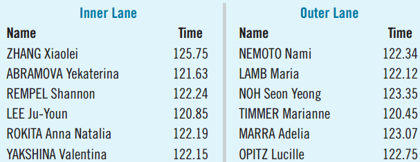
• Speed-skating races run in pairs. One starts in the inner lane, the other in the outer lane.
• Above are some of the randomly assigned pairs.
• The data are paired rather than independent.
• Blocking involves pairing arising from an experiment.
• Matching involves pairing arising from an observational study.
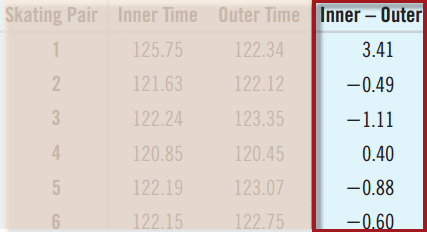
• With pairing, we look at the differences.

Differences for Speed-Skater Pairs

• For paired data, create a new data set of the differences.
• We can now look only at the differences.
• Ignoring the original data, we now have a single data set.

• Proceed with a one-sample t-test. This process is called a paired t-test.
• Only use pairing if there is a natural matching

The Paired t-Test

When the conditions are met, we can test whether the mean differences significantly differ from 0.

• H₀: \(\mu_d = \Delta_0\) (\(\Delta_0\) is usually 0)

\[t = \frac{\bar{d} - \Delta_0}{SE\left(\bar{d}\right)} \qquad SE\left(\bar{d}\right) = \frac{s_d}{\sqrt{n}}\]

• \(\bar{d}\) and s_d are the mean and standard deviation of the pairwise differences and n is the number of pairs.
• Use the Student’s t-model with n – 1 degrees of freedom and find the P-value.

Speed-Skating Comparisons

Was there a difference between speeds between inner and outer speed-skating lanes?

• Plan: I have data for 17 pairs of racers.
• Hypotheses:
  • H₀: \(\mu_d = 0\)
  • H_A: \(\mu_d \ne 0\)

Speed-Skating Comparisons

• Mechanics:

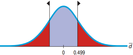
n = 17 pairs, \(\bar{d}\) = 0.499 sec., s_d = 2.333 sec.

\[SE\left(\bar{d}\right) = \frac{s_d}{\sqrt{n}} = \frac{2.333}{\sqrt{17}} = 0.5658\]

\[t_{16} = \frac{\bar{d} - 0}{SE\left(\bar{d}\right)} = \frac{0.499}{0.5658} \approx 0.882\]

\[\text{P-value} = 2P(t_{16} > 0.882) = 0.39\]

Speed-Skating Comparisons

• Conclusion:
  • Events that occur more than a third of the time (P-value = 0.39) are not remarkable.
  • I can’t conclude that the observed difference isn’t due simply to random chance. It appears the fans may have interpreted a random fluctuation in the data as favoring one lane. There’s insufficient evidence to declare any lack of fairness.

Paired t-interval

When the conditions are met, the confidence interval for the mean paired difference is

\[\bar{d} \pm t^{*}_{n-1} \times SE\left(\bar{d}\right) \qquad SE\left(\bar{d}\right) = \frac{s_d}{\sqrt{n}}\]

• The critical value t* from the Student’s t-model depends on the confidence level C and df = n – 1. (n is the number of pairs.)

Inference for counts

Review: Chi-Square test for count data

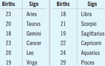
• A single basis of classification: Goodness of fit
• df: n-1, where n is the number of categories
• I have a model and I am checking its validity
• Two variables: Homogeneity
• The counts are the results of some process. Are the counts the same for every cell?
• Two variables: Independence
• If factors independent I should have same proportion across cells

Example 1: Are CEO Zodiac Signs Uniform?

• A survey of 256 randomly selected CEOs’ Zodiac signs
• If uniform, each sign expected to have 256/12 ≈ 21.3 births
• Pisces has more.
• Others have fewer.
• Is the distribution far enough from uniform to conclude the data do not come from a uniform distribution?

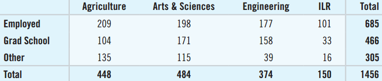
Example 2: Activities of Graduates at Different Colleges

• Are graduates’ activities the same at different colleges within the same university?

Example 3: Tattoos and Hepatitis

Are Tattoo Status and Hepatitis Status independent?

• Plan: Test for independence. I have a contingency table of 626 patients.
• Hypotheses:
  • H₀: Tattoo Status and Hepatitis Status are independent.
  • H_A: Tattoo Status and Hepatitis Status are not independent.

Chi-Square Calculations

• Interested in the differences between observed and expected counts: called residuals.
• Make positive by squaring them all.
• Get relative sizes of the residuals by dividing them by the expected counts.

\[\chi^2 = \sum \frac{\left(Obs - Exp\right)^2}{Exp}\]

• This is a Chi-Square Model with df = n – 1.
• n is the number of categories, not the sample size.

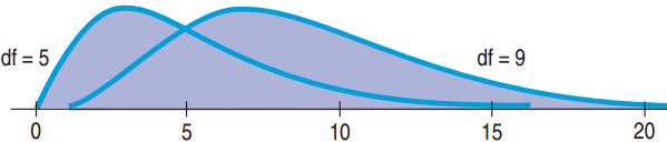
Why so big? The Shape of \(\chi^2\)

• With df large (more cells), the weighted residuals add up quickly → numerator gets bigger
• Unlike z or t, a larger \(\chi^2\) is more common. It all depends on the df: look at value 10
• The mode of \(\chi^2\) is df – 2.
• The expected value of \(\chi^2\) is df, to the right of the mode due to the right skewed distribution.
• The CEO curve had df=11, peaks at 9 and mean=11

Inference for regression

Body Fat and Waist Size

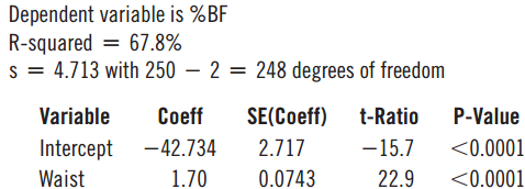
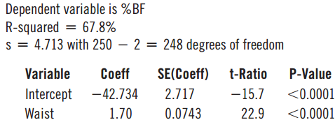
• Mechanics: Computer Output:

• The estimated regression equation is:

\[\widehat{\%Body\ Fat} = -42.73 + 1.70\ Waist\]

Testing for \(\beta_1\)

• With no linear association, \(\beta_1 = 0\)
• H₀: \(\beta_1 = 0\)

\[t_{n-2} = \frac{b_1 - 0}{SE\left(b_1\right)}\]

• For the %Body Fat and Waist data:

\[\frac{1.7 - 0}{0.0743} \approx 22.9 \qquad \text{P-value} < 0.0001\]

• Very unlikely to have such a high b₁ if \(\beta_1 = 0\)

Confidence Interval for \(\beta_1\)

• The hypothesis test for %Body Fat and Waist told us what we already know.
• A confidence interval is needed.

\[b_1 \pm t^{*}_{n-2} \times SE(b_1)\]

• For %Body Fat and Waist:
  • 1.7 ± 1.97 × 0.074 = (1.55%, 1.85%)
• With 95% confidence the slope of the line for %Body Fat and Waist is between 1.55% and 1.85%.

Analysis of Variance

Back to Bacteria

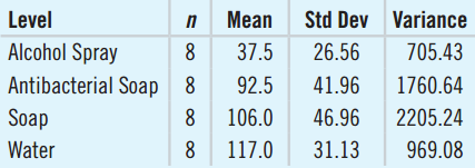
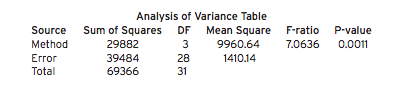
• MS_T = 9960.64, MS_E = 1410.14

\[F = \frac{MS_T}{MS_E} = \frac{9960.64}{1410.14} \approx 7.06\]

• Num df = 4 – 1 = 3, Den df = 4(8 – 1) = 28.
• Technology gives P-value for F_3,28 = 0.0011.

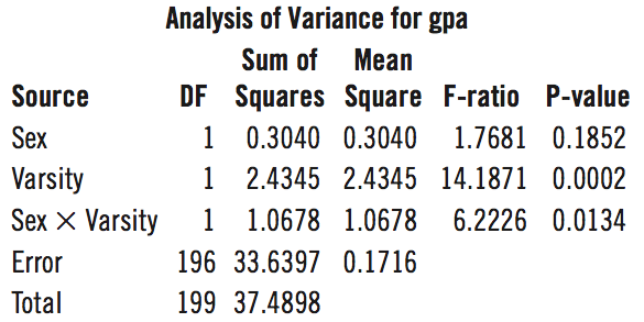
Example: Two-Factor ANOVA with Interaction Step-By-Step

Plan – Show the ANOVA table.

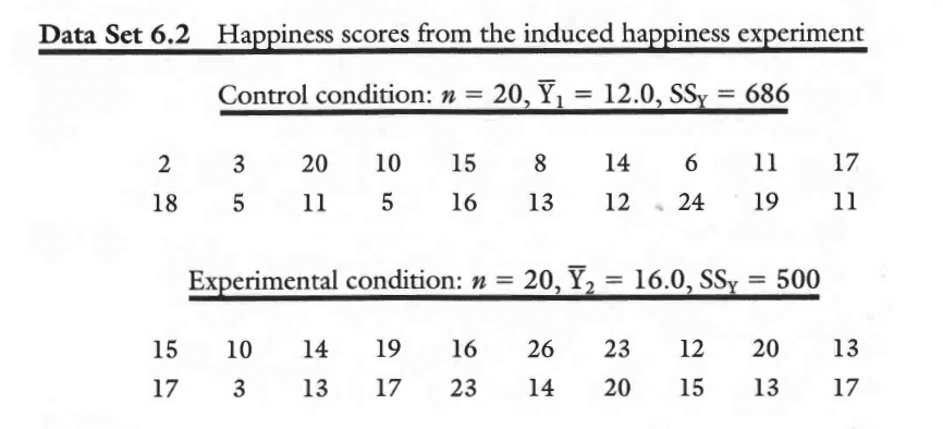
This experiment is modeled after one reported by Laird (1974). The experiment asks whether an induced smile actually has the effect of making a person feel happier. In the experimental condition, participants were instructed to move facial muscles to mimic a smile while looking at a picture of children playing. In a second control condition, participants simply looked at the picture with a neutral facial expression. No mention was made of smiling to any of the participants; participants believed the purpose of the experiment was to evaluate the effect of facial muscles on perception. A total of 40 volunteers participated in the experiment. They were assigned randomly to the two conditions, 20 participants in each. The response measure was a “happiness score” obtained by administering a mood questionnaire.

Calculate the 95% and the 99% confidence intervals.

Suppose a simple random sample of 150 students is drawn from a population of 3000 college students. Among sampled students, the average IQ score is 115 with a standard deviation of 10. What is the 99% confidence interval for the students’ IQ score?

For boys, the average number of absences in the first grade is 15 with a standard deviation of 7; for girls, the average number of absences is 10 with a standard deviation of 6.

In a nationwide survey, suppose 100 boys and 50 girls are sampled. What is the probability that the male sample will have at most three more days of absences than the female sample?